Utilisation de l'interférence Bayésienne pour la génération de ShakeMaps

Présentation de Pierre Gehl (BRGM) au 2nd Workshop Résif "Aléa sismique & Shakemaps" | 29 - 31 janvier 2018, Montpellier

Transcript

1. Utilisation de l’inférence Bayésienne pour la génération de ShakeMaps Pierre Gehl – BRGM Avec John Douglas – University of Strathclyde Dina D’Ayala – University College London 2nd Workshop RESIF – Aléa sismique & Shakemaps Shakemap – Alternatives méthodologiques
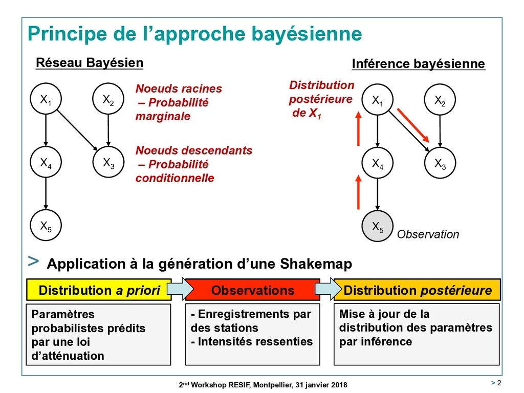
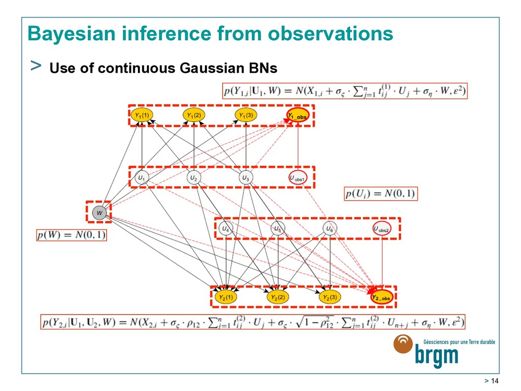
2. > 2 Principe de l’approche bayésienne 2nd Workshop RESIF, Montpellier, 31 janvier 2018 X1 X2 X3 X4 X5 Réseau Bayésien Noeuds racines – Probabilité marginale Noeuds descendants – Probabilité conditionnelle X1 X2 X3 X4 X5 Observation Distribution postérieure de X1 Inférence bayésienne >  Application à la génération d’une Shakemap Distribution a priori Observations Distribution postérieure Paramètres probabilistes prédits par une loi d’atténuation - Enregistrements par des stations - Intensités ressenties Mise à jour de la distribution des paramètres par inférence
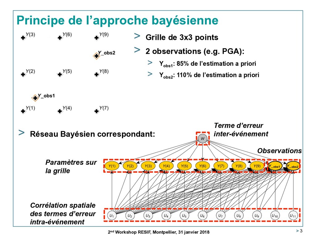
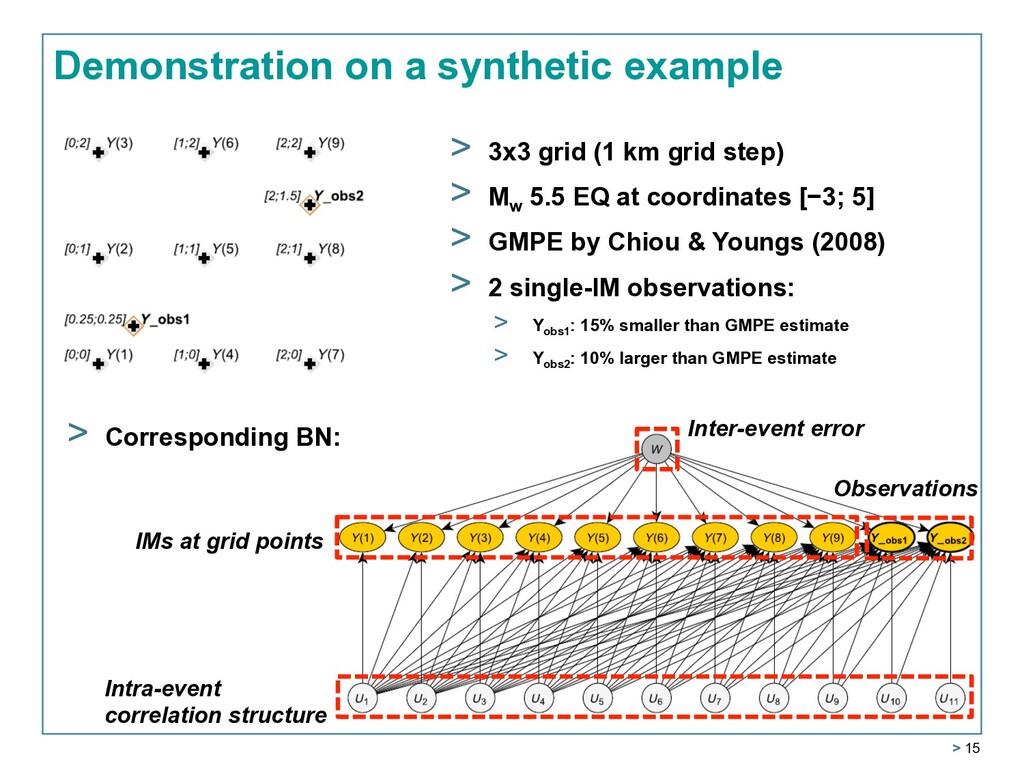
3. > 3 Principe de l’approche bayésienne 2nd Workshop RESIF, Montpellier, 31 janvier 2018 >  Grille de 3x3 points >  2 observations (e.g. PGA): >  Yobs1 : 85% de l’estimation a priori >  Yobs2 : 110% de l’estimation a priori >  Réseau Bayésien correspondant: Terme d’erreur inter-événement Paramètres sur la grille Corrélation spatiale des termes d’erreur intra-événement Observations
4. > 4 Principe de l’approche bayésienne 2nd Workshop RESIF, Montpellier, 31 janvier 2018 Terme global (inter-événement) Terme local (intra- événement) Terme local (intra- événement)
5. > 5 Traitement de plusieurs types d’observations 2nd Workshop RESIF, Montpellier, 31 janvier 2018 GMICE SA(T) PGA GMPE MMI GMPE Corrélation spatiale PGA Corrélation spatiale SA(T)
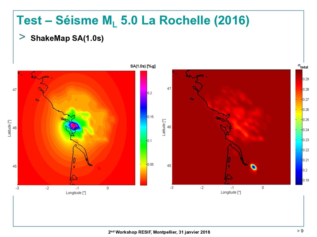
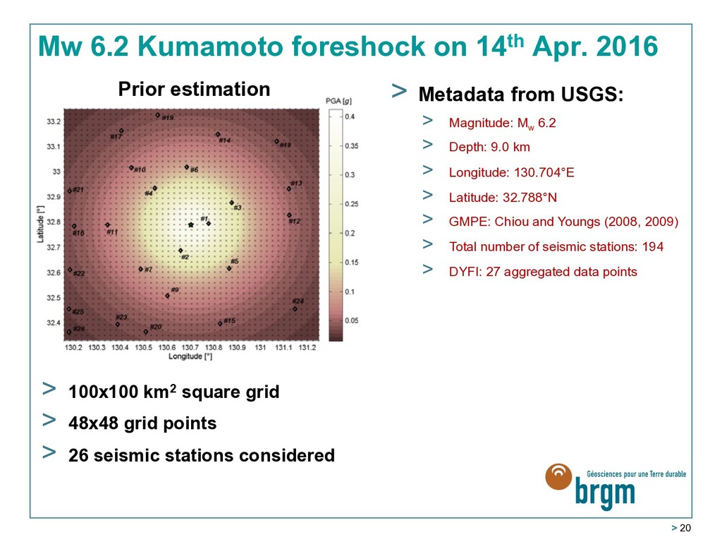
6. > 6 Validation – Séisme Mw 6.2 Kumamoto (2016) 2nd Workshop RESIF, Montpellier, 31 janvier 2018 PGA [g] SA(1.0s) [g] >  Grille de 48x48 points (100x100 km2) >  26 stations sismiques >  Estimation conjointe de PGA et SA(1.0s) >  Résultats quasi-identiques à l’approche ShakeMap USGS >  Traitement rigoureux de l’incertitude (équilibre entre les variabilités inter- et intra-événement) cf. Gehl et al. (2017) pour la validation analytique
7. > 7 Test – Séisme ML 5.0 La Rochelle (2016) 2nd Workshop RESIF, Montpellier, 31 janvier 2018 >  Peu d’observations intrumentales (2 stations) >  Nombreux témoignages (370 observations utilisées) >  ShakeMap en Intensité:
8. > 8 Test – Séisme ML 5.0 La Rochelle (2016) 2nd Workshop RESIF, Montpellier, 31 janvier 2018 >  ShakeMap PGA: 0.7% g (Franceséisme) 1.4% g (Franceséisme)
9. > 9 Test – Séisme ML 5.0 La Rochelle (2016) 2nd Workshop RESIF, Montpellier, 31 janvier 2018 >  ShakeMap SA(1.0s)
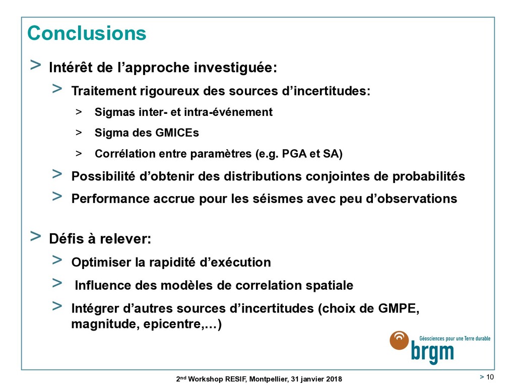
10. > 10 Conclusions >  Intérêt de l’approche investiguée: >  Traitement rigoureux des sources d’incertitudes: >  Sigmas inter- et intra-événement >  Sigma des GMICEs >  Corrélation entre paramètres (e.g. PGA et SA) >  Possibilité d’obtenir des distributions conjointes de probabilités >  Performance accrue pour les séismes avec peu d’observations >  Défis à relever: >  Optimiser la rapidité d’exécution >  Influence des modèles de correlation spatiale >  Intégrer d’autres sources d’incertitudes (choix de GMPE, magnitude, epicentre,…) 2nd Workshop RESIF, Montpellier, 31 janvier 2018
11. > 11 Références Bensi, M.T., Der Kiureghian, A. and Straub, D. (2011). A Bayesian Network methodology for infrastructure seismic risk assessment and decision support. PEER Report 2011/02, Berkeley, California. Gehl, P., Douglas, J., & D'Ayala, D. (2017). Inferring Earthquake Ground-Motion Fields with Bayesian Networks. Bulletin of the Seismological Society of America, 107(6), 2792-2808. Murphy, K. (2007). Bayes Net toolbox. Available from https://github.com/bayesnet/bnt. 2nd Workshop RESIF, Montpellier, 31 janvier 2018
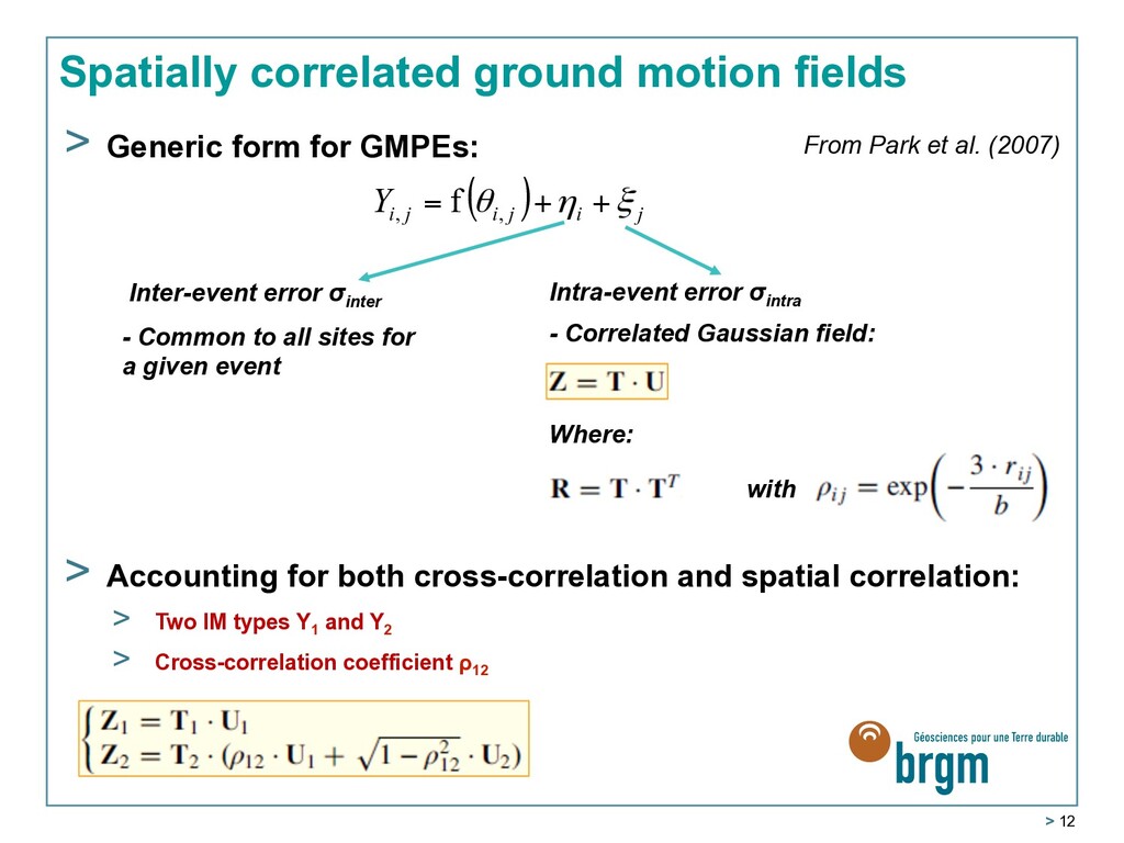
12. > 12 Spatially correlated ground motion fields >  Generic form for GMPEs: ( ) j i j i j i Y ξ η θ + + = , , f Inter-event error σinter Intra-event error σintra - Correlated Gaussian field: - Common to all sites for a given event >  Accounting for both cross-correlation and spatial correlation: >  Two IM types Y1 and Y2 >  Cross-correlation coefficient ρ12 Where: with From Park et al. (2007)
13. > 13 General principles of Bayesian Networks >  BN = acyclic oriented graph è nodes (variables) and oriented edges (statistical dependencies) >  Discrete or continuous Gaussian variables X1 X2 X3 X4 X5 Root nodes – Marginal probability Child node – Conditional probability X1 X2 X3 X4 X5 Evidence Posterior distribution of X1 BN inference BN structure
14. > 14 Bayesian inference from observations >  Use of continuous Gaussian BNs
15. > 15 Demonstration on a synthetic example >  3x3 grid (1 km grid step) >  Mw 5.5 EQ at coordinates [−3; 5] >  GMPE by Chiou & Youngs (2008) >  2 single-IM observations: >  Yobs1 : 15% smaller than GMPE estimate >  Yobs2 : 10% larger than GMPE estimate >  Corresponding BN: Inter-event error IMs at grid points Intra-event correlation structure Observations
16. > 16 Demonstration on a synthetic example >  Junction-tree algorithm: >  Updating of the probability distributions:
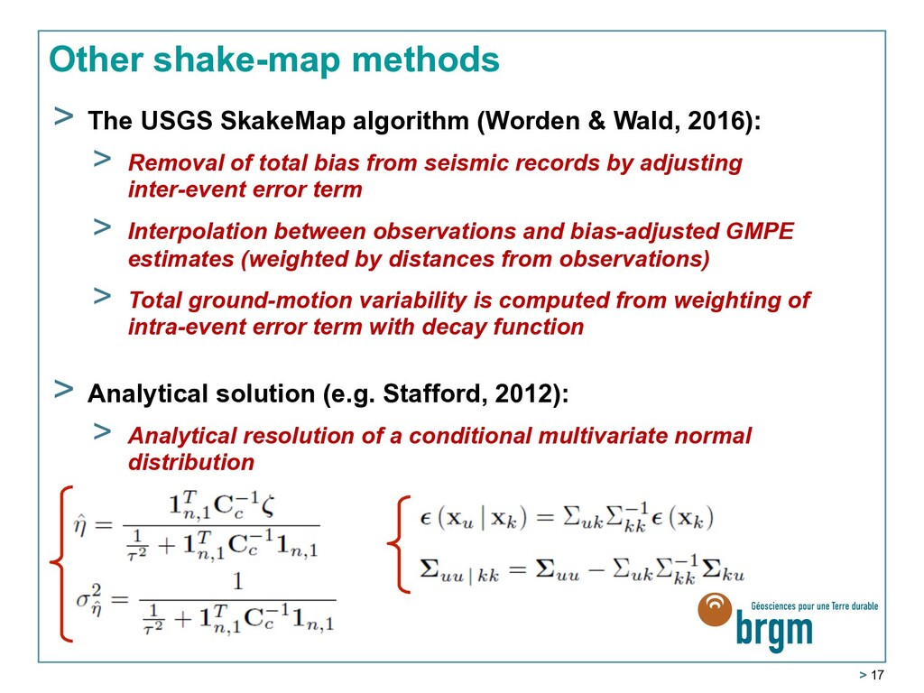
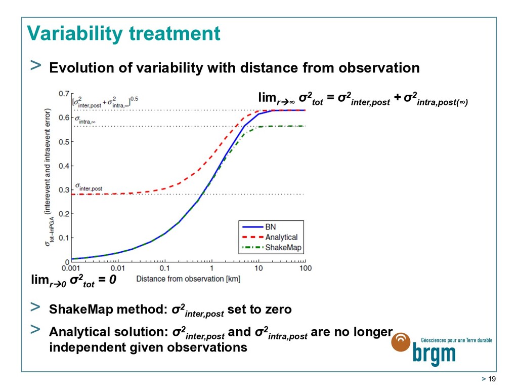
17. > 17 Other shake-map methods >  The USGS SkakeMap algorithm (Worden & Wald, 2016): >  Removal of total bias from seismic records by adjusting inter-event error term >  Interpolation between observations and bias-adjusted GMPE estimates (weighted by distances from observations) >  Total ground-motion variability is computed from weighting of intra-event error term with decay function >  Analytical solution (e.g. Stafford, 2012): >  Analytical resolution of a conditional multivariate normal distribution
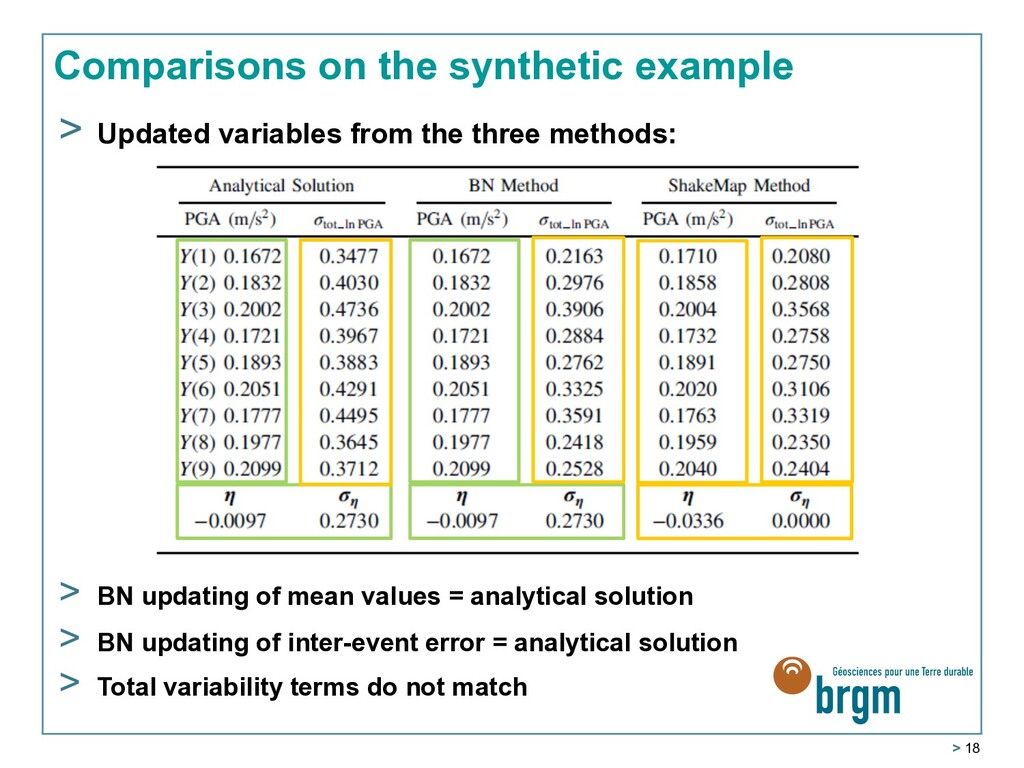
18. > 18 Comparisons on the synthetic example >  Updated variables from the three methods: >  BN updating of mean values = analytical solution >  BN updating of inter-event error = analytical solution >  Total variability terms do not match
19. > 19 Variability treatment >  Evolution of variability with distance from observation limrà∞ σ2 tot = σ2 inter,post + σ2 intra,post(∞) limrà0 σ2 tot = 0 >  ShakeMap method: σ2 inter,post set to zero >  Analytical solution: σ2 inter,post and σ2 intra,post are no longer independent given observations
20. > 20 Mw 6.2 Kumamoto foreshock on 14th Apr. 2016 Prior estimation >  Metadata from USGS: >  Magnitude: Mw 6.2 >  Depth: 9.0 km >  Longitude: 130.704°E >  Latitude: 32.788°N >  GMPE: Chiou and Youngs (2008, 2009) >  Total number of seismic stations: 194 >  DYFI: 27 aggregated data points >  100x100 km2 square grid >  48x48 grid points >  26 seismic stations considered
21. > 21 Single-IM Bayesian inference PGA shake-map Uncertainty on ln(PGA) BN approach ShakeMap algorithm
22. > 22 Joint inference of cross-correlated IMs PGA [g] SA(1.0s) [g] >  Ability to compute joint probabilities at a given site >  Helpful for the assessment of infrastructure systems affected by multiple types of IM >  Seismic stations with missing data can still be used to constrain the ground-motion field
23. > 23 Accounting for macroseismic observations PGA [g] MMI >  200x200 km2 square grid >  96x96 grid points >  90 seismic stations considered + 14 macroseismic observations è ~ 1 hour of processing time on a (slow) personal computer