Kingdom Modelling site-disordered solids: new developments and applications using the SOD package Winter School on Modelling and Simulations of Materials for Energy and the Environment JNCASR, Bangalore, December 2018
postgraduate studies at the University of Reading. • Covers all tuition fees at international rate and stipend (currently £14k per year). Also allowances for clothes, books and a return flight home. • Candidates must have a first-class degree from an Indian university, and demonstrate financial need. • Deadline for programmes starting in September 2019: candidates must hold an offer of admission by 30th January 2019. https://www.reading.ac.uk/gs-felix.aspx
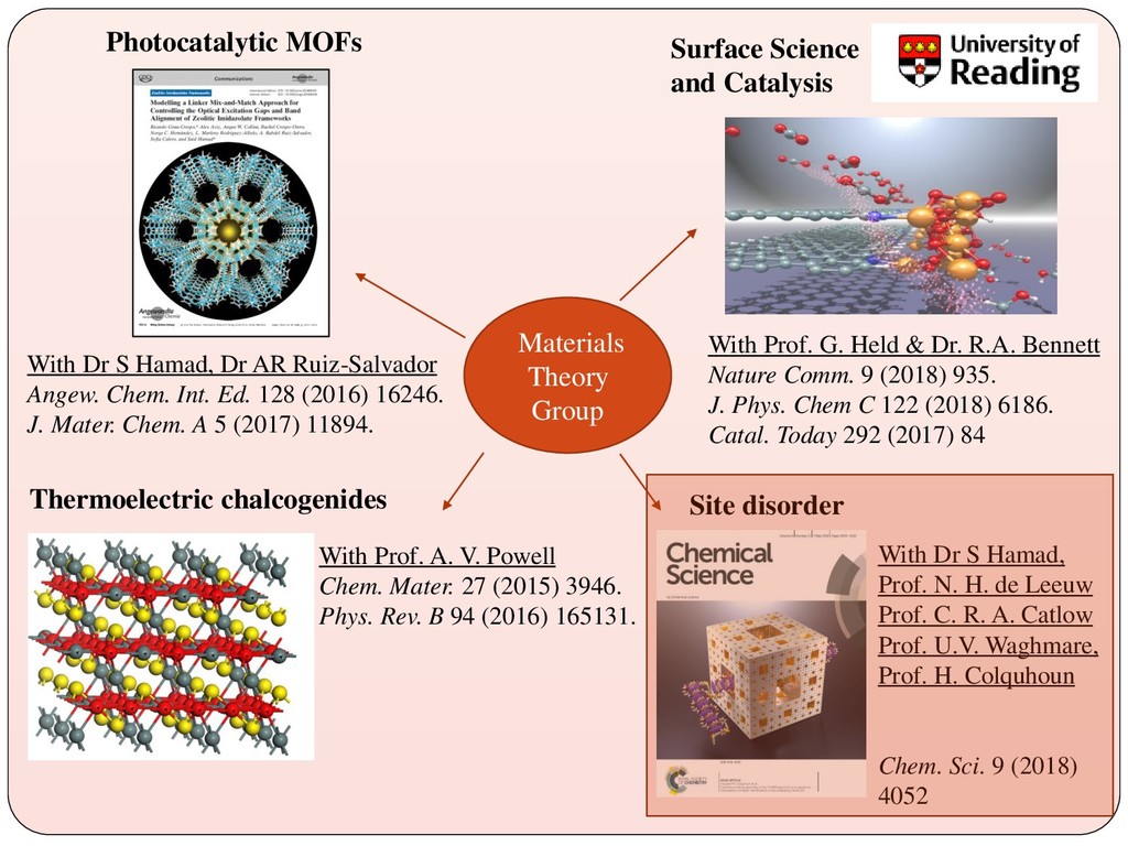
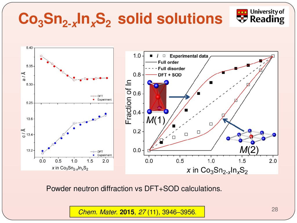
MOFs Site disorder With Prof. G. Held & Dr. R.A. Bennett Nature Comm. 9 (2018) 935. J. Phys. Chem C 122 (2018) 6186. Catal. Today 292 (2017) 84 With Dr S Hamad, Dr AR Ruiz-Salvador Angew. Chem. Int. Ed. 128 (2016) 16246. J. Mater. Chem. A 5 (2017) 11894. With Prof. A. V. Powell Chem. Mater. 27 (2015) 3946. Phys. Rev. B 94 (2016) 165131. With Dr S Hamad, Prof. N. H. de Leeuw Prof. C. R. A. Catlow Prof. U.V. Waghmare, Prof. H. Colquhoun Chem. Sci. 9 (2018) 4052
of methods - The Site Occupancy Disorder (SOD) method. - Examples of applications: cation distributions at the bulk and surfaces of materials - Extension to grand-canonical ensembles. - Beyond thermodynamics: averaging NMR spectra. - Speeding up energy evaluations using ab-initio-defined pair- wise interactions
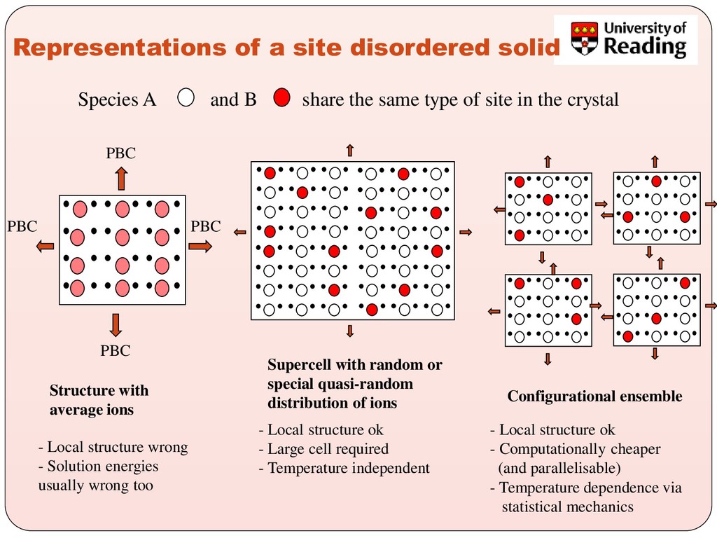
share the same type of site in the crystal PBC Structure with average ions PBC PBC PBC - Local structure wrong - Solution energies usually wrong too Supercell with random or special quasi-random distribution of ions - Local structure ok - Large cell required - Temperature independent Configurational ensemble - Local structure ok - Computationally cheaper (and parallelisable) - Temperature dependence via statistical mechanics
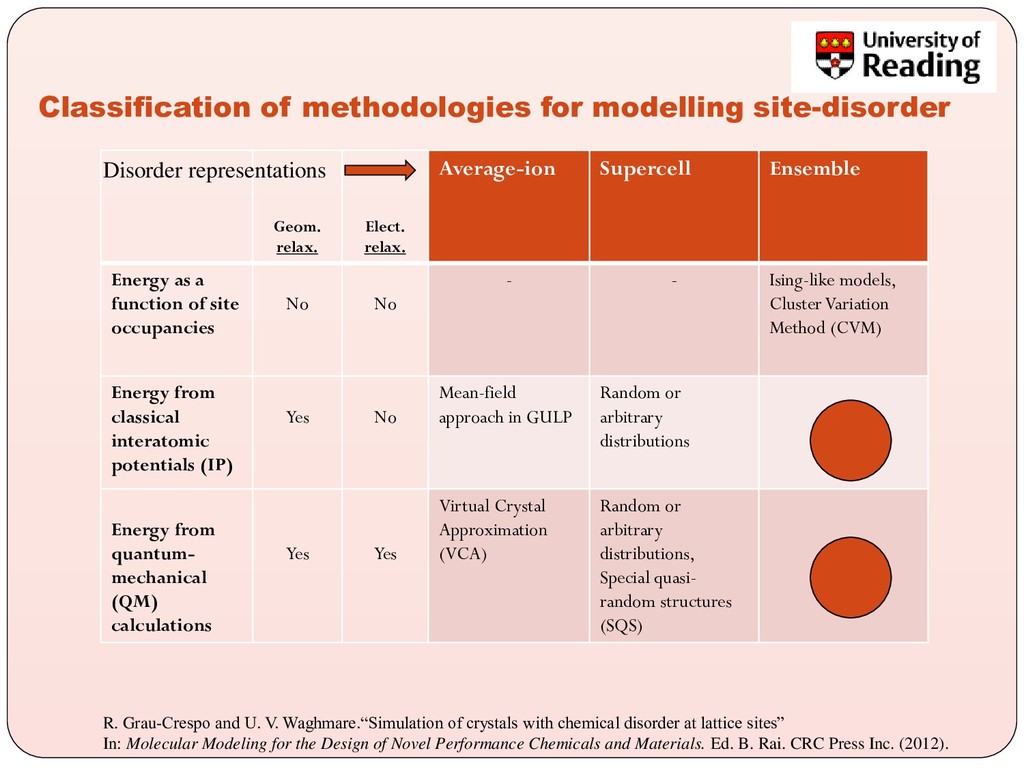
Average-ion Supercell Ensemble Energy as a function of site occupancies No No - - Ising-like models, ClusterVariation Method (CVM) Energy from classical interatomic potentials (IP) Yes No Mean-field approach in GULP Random or arbitrary distributions Energy from quantum- mechanical (QM) calculations Yes Yes Virtual Crystal Approximation (VCA) Random or arbitrary distributions, Special quasi- random structures (SQS) Disorder representations R. Grau-Crespo and U. V. Waghmare.“Simulation of crystals with chemical disorder at lattice sites” In: Molecular Modeling for the Design of Novel Performance Chemicals and Materials. Ed. B. Rai. CRC Press Inc. (2012).
are difficult to parameterise in cluster expansion models (e.g. long-range interactions in ionic solids, strong geometric relaxations, changes in electronic configurations, etc.) - IP and QM methods provide not just energies but also other properties for each configuration (e.g. local geometries and cell parameters, electronic structure, spectra). Configurational averages can then be obtained. - They allow to directly evaluate vibrational properties of the disordered solid. - They also allow to extend the simulations to solid surfaces, which is difficult with simpler interaction models.
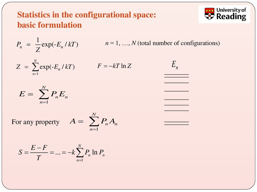
n n E P E = = n E 1 ... ln N n n n E F S k P P T = − = = = − n = 1, …, N (total number of configurations) 1 exp(- / ) n n P E kT Z = 1 exp(- / ) N n n Z E kT = = ln F kT Z = − 1 N n n n A P A = = For any property
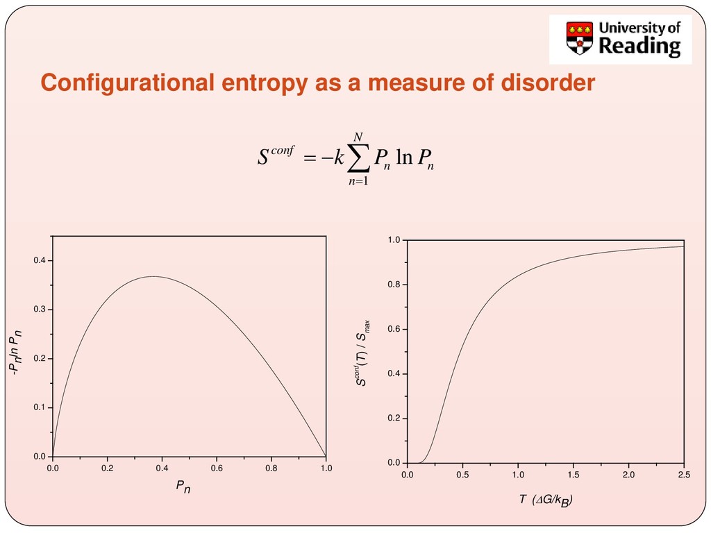
conf n n n S k P P = = − 0.0 0.2 0.4 0.6 0.8 1.0 0.0 0.1 0.2 0.3 0.4 -Pnln Pn Pn 0.0 0.5 1.0 1.5 2.0 2.5 0.0 0.2 0.4 0.6 0.8 1.0 Sconf(T) / S max T (G/kB)
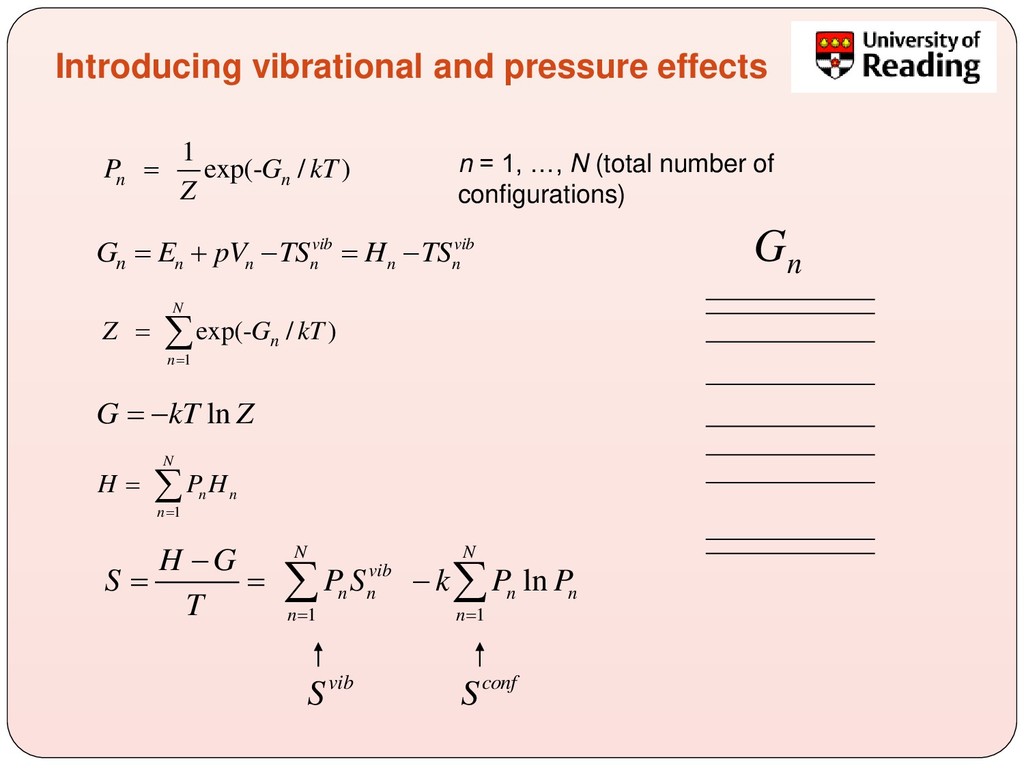
= n = 1, …, N (total number of configurations) vib vib n n n n n n G E pV TS H TS = + − = − 1 exp(- / ) N n n Z G kT = = ln G kT Z = − 1 N n n n H P H = = 1 1 ln N N vib n n n n n n H G S P S k P P T = = − = = − conf S vib S n G Introducing vibrational and pressure effects
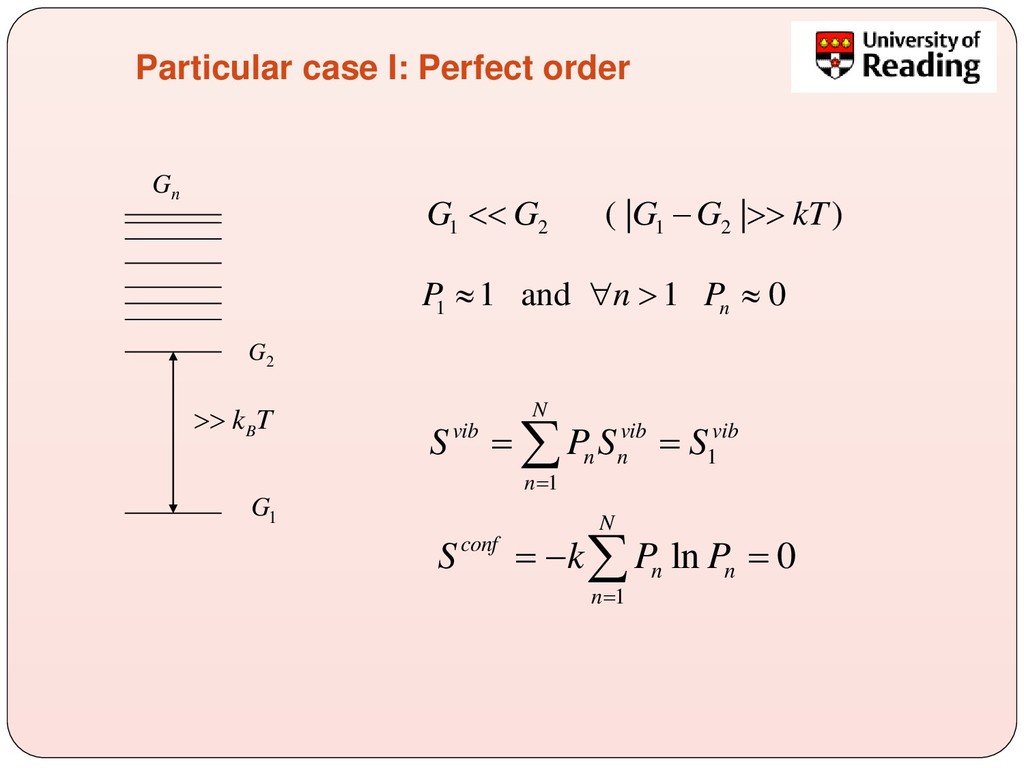
k T 1 2 1 2 ( | | ) G G G G kT − 2 G 1 1 and 1 0 n P n P 1 1 N vib vib vib n n n S P S S = = = 1 ln 0 N conf n n n S k P P = = − =
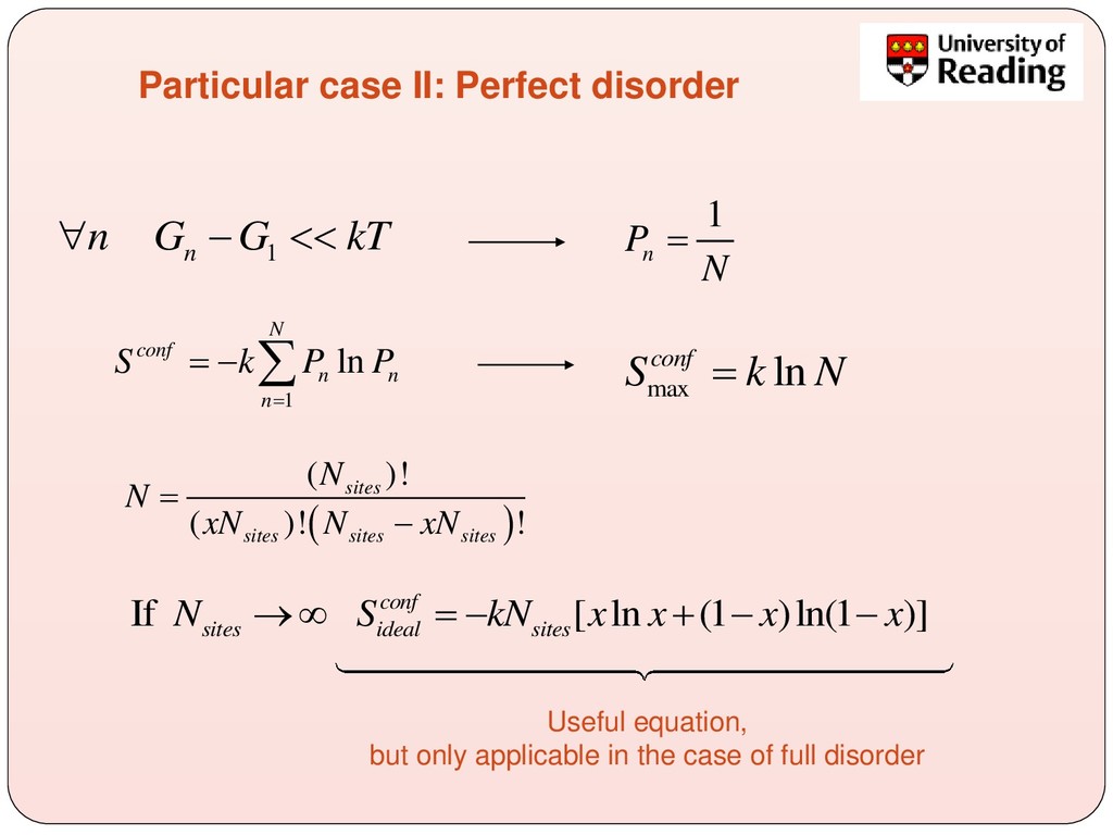
n n S k P P = = − max ln conf S k N = 1 n n G G kT − 1 n P N = ( ) ( )! ( )! ! sites sites sites sites N N xN N xN = − If [ ln (1 )ln(1 )] conf sites ideal sites N S kN x x x x → = − + − − Useful equation, but only applicable in the case of full disorder
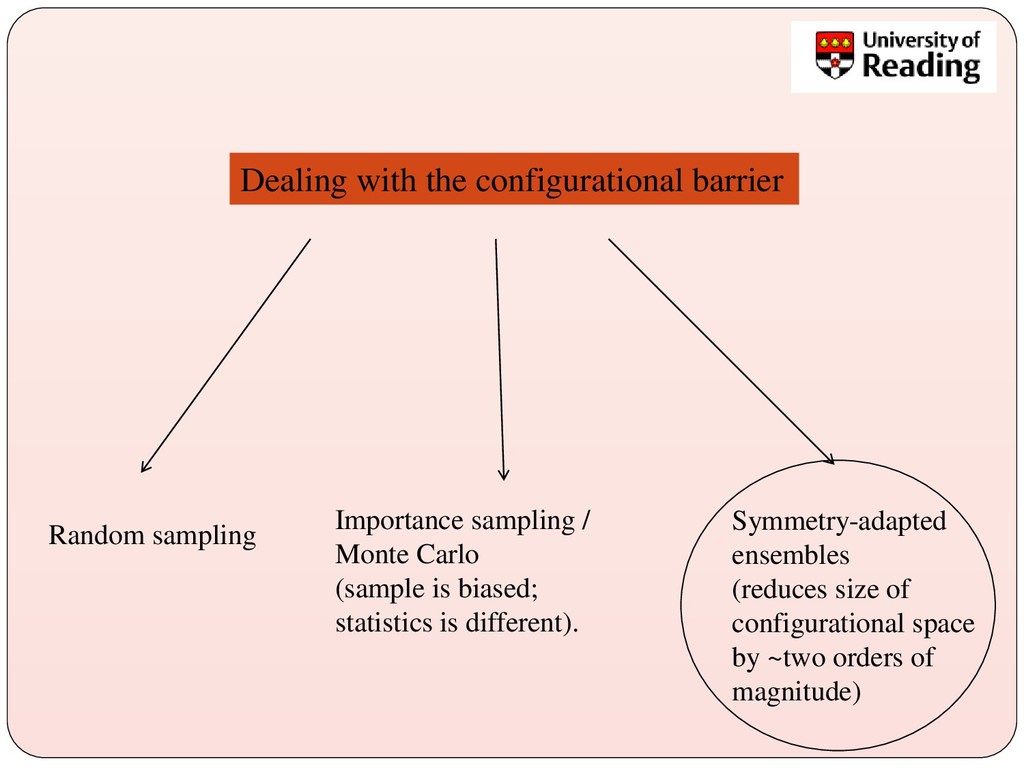
Monte Carlo (sample is biased; statistics is different). Symmetry-adapted ensembles (reduces size of configurational space by ~two orders of magnitude)
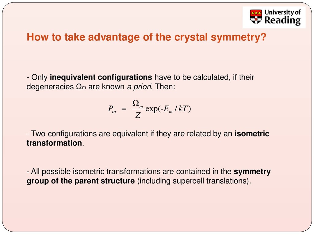
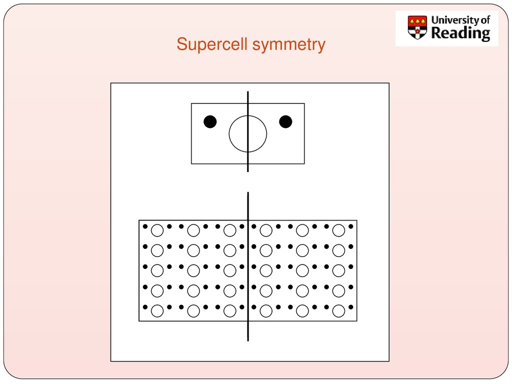
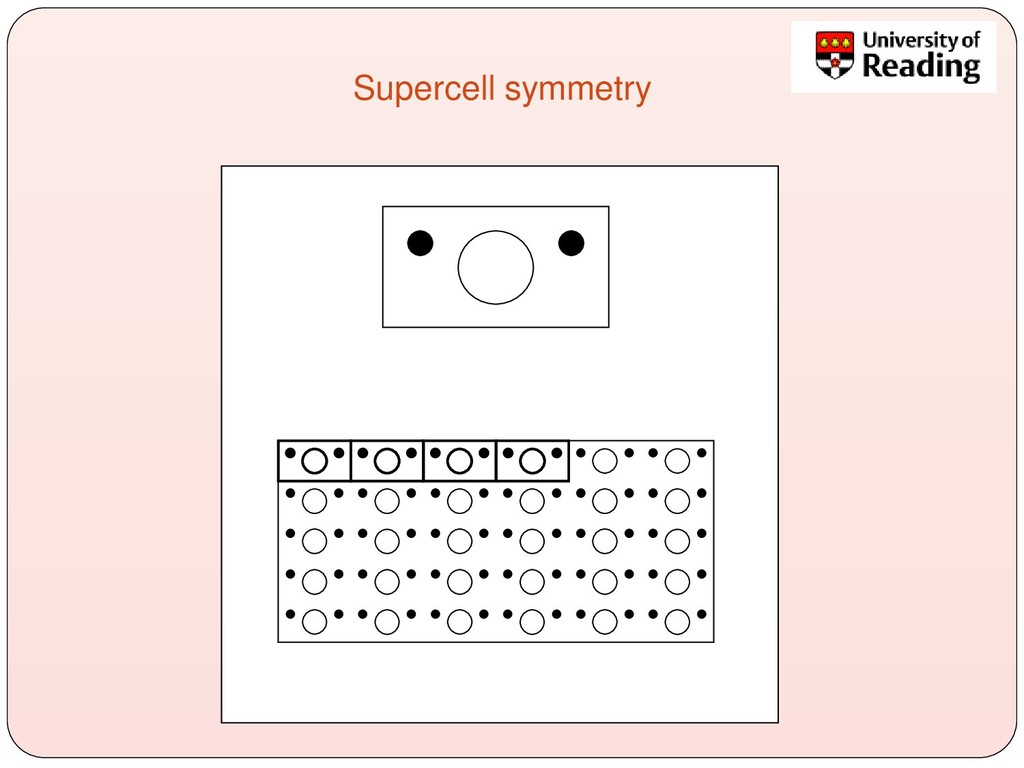
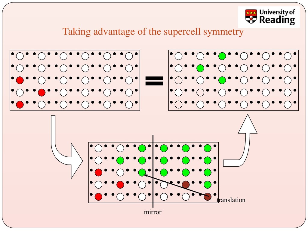
inequivalent configurations have to be calculated, if their degeneracies Ωm are known a priori. Then: - Two configurations are equivalent if they are related by an isometric transformation. - All possible isometric transformations are contained in the symmetry group of the parent structure (including supercell translations). exp(- / ) m m m P E kT Z =
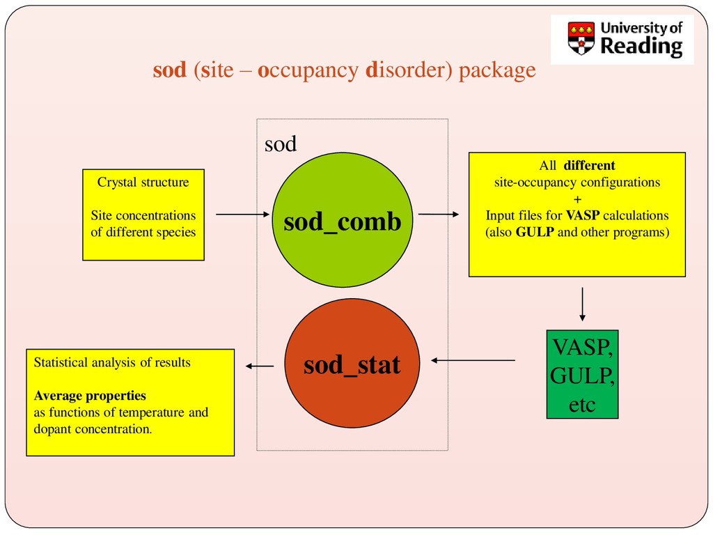
concentrations of different species All different site-occupancy configurations + Input files for VASP calculations (also GULP and other programs) sod_stat Statistical analysis of results Average properties as functions of temperature and dopant concentration. VASP, GULP, etc sod
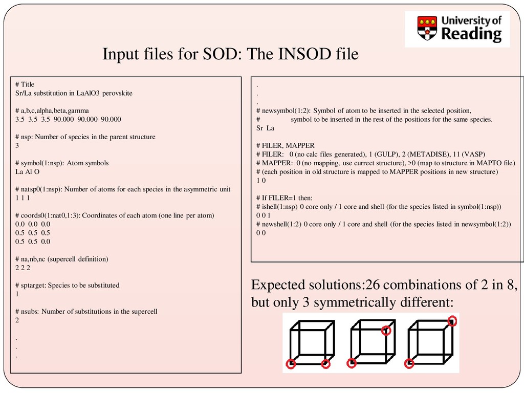
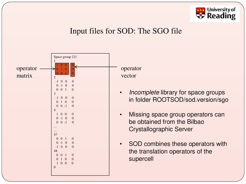
substitution in LaAlO3 perovskite # a,b,c,alpha,beta,gamma 3.5 3.5 3.5 90.000 90.000 90.000 # nsp: Number of species in the parent structure 3 # symbol(1:nsp): Atom symbols La Al O # natsp0(1:nsp): Number of atoms for each species in the asymmetric unit 1 1 1 # coords0(1:nat0,1:3): Coordinates of each atom (one line per atom) 0.0 0.0 0.0 0.5 0.5 0.5 0.5 0.5 0.0 # na,nb,nc (supercell definition) 2 2 2 # sptarget: Species to be substituted 1 # nsubs: Number of substitutions in the supercell 2 . . . . . . # newsymbol(1:2): Symbol of atom to be inserted in the selected position, # symbol to be inserted in the rest of the positions for the same species. Sr La # FILER, MAPPER # FILER: 0 (no calc files generated), 1 (GULP), 2 (METADISE), 11 (VASP) # MAPPER: 0 (no mapping, use currect structure), >0 (map to structure in MAPTO file) # (each position in old structure is mapped to MAPPER positions in new structure) 1 0 # If FILER=1 then: # ishell(1:nsp) 0 core only / 1 core and shell (for the species listed in symbol(1:nsp)) 0 0 1 # newshell(1:2) 0 core only / 1 core and shell (for the species listed in newsymbol(1:2)) 0 0 Expected solutions:26 combinations of 2 in 8, but only 3 symmetrically different:
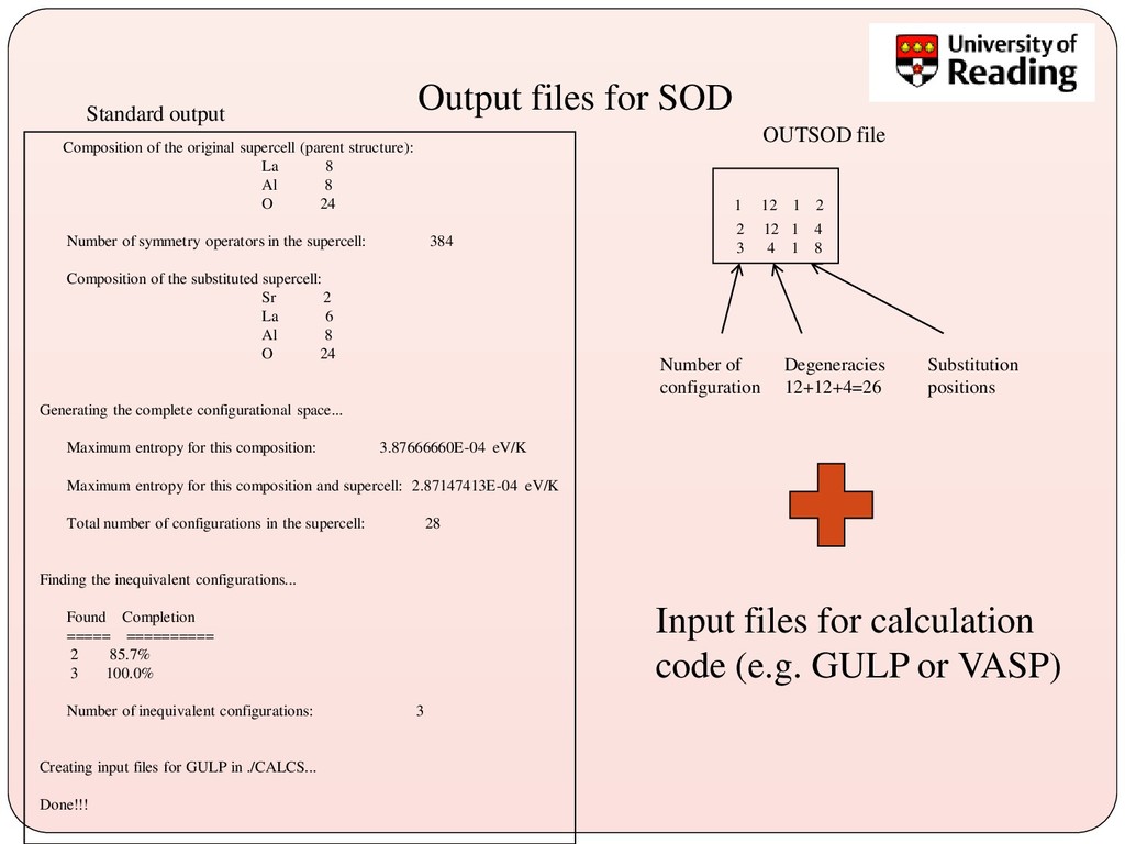
structure): La 8 Al 8 O 24 Number of symmetry operators in the supercell: 384 Composition of the substituted supercell: Sr 2 La 6 Al 8 O 24 Generating the complete configurational space... Maximum entropy for this composition: 3.87666660E-04 eV/K Maximum entropy for this composition and supercell: 2.87147413E-04 eV/K Total number of configurations in the supercell: 28 Finding the inequivalent configurations... Found Completion ===== ========== 2 85.7% 3 100.0% Number of inequivalent configurations: 3 Creating input files for GULP in ./CALCS... Done!!! Standard output OUTSOD file 1 12 1 2 2 12 1 4 3 4 1 8 Number of configuration Degeneracies 12+12+4=26 Substitution positions Input files for calculation code (e.g. GULP or VASP)
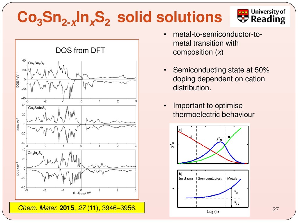
S2 solid solutions DOS from DFT • metal-to-semiconductor-to- metal transition with composition (x) • Semiconducting state at 50% doping dependent on cation distribution. • Important to optimise thermoelectric behaviour
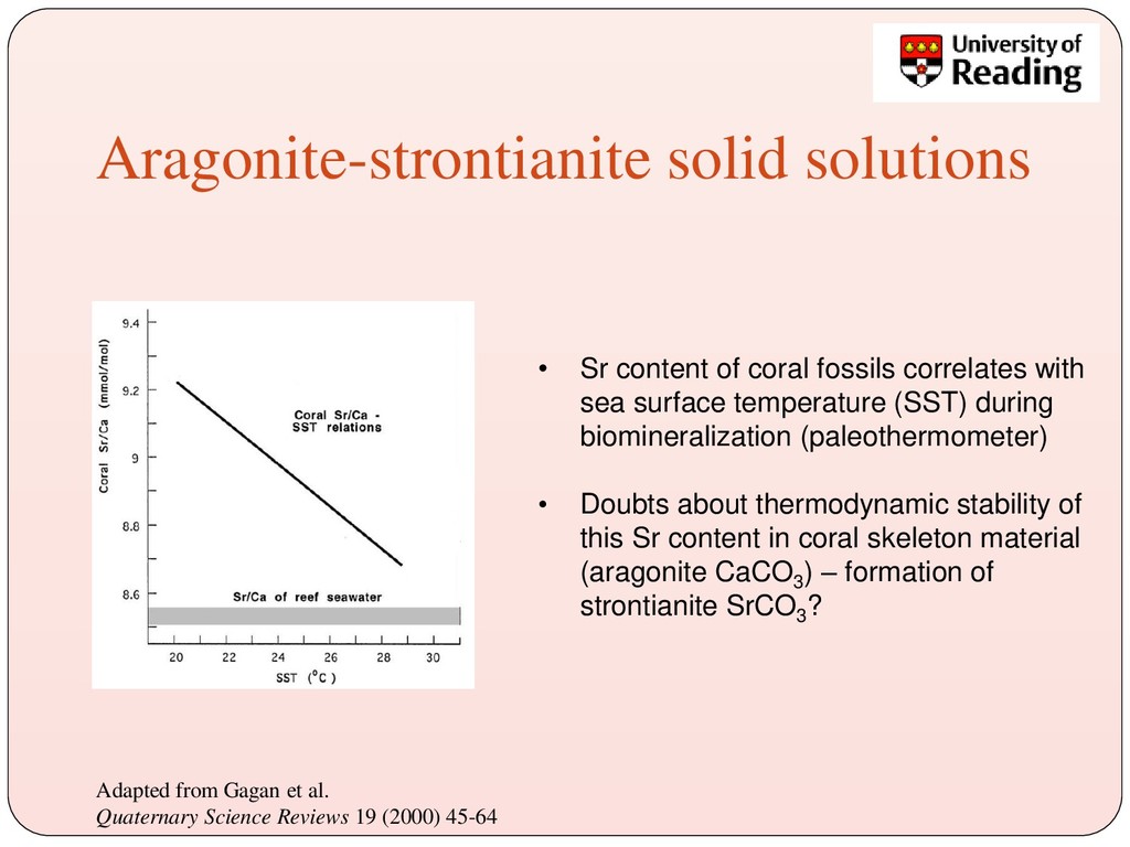
Reviews 19 (2000) 45-64 • Sr content of coral fossils correlates with sea surface temperature (SST) during biomineralization (paleothermometer) • Doubts about thermodynamic stability of this Sr content in coral skeleton material (aragonite CaCO3 ) – formation of strontianite SrCO3 ?
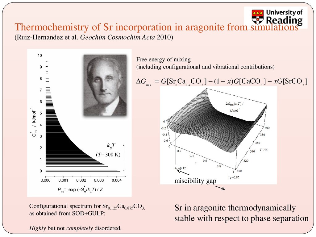
al. Geochim Cosmochim Acta 2010) Configurational spectrum for Sr0.125 Ca0.875 CO3, as obtained from SOD+GULP: Highly but not completely disordered. mix 1- 3 3 3 [Sr Ca CO ] (1 ) [CaCO ] [SrCO ] x x G G x G xG = − − − miscibility gap Free energy of mixing (including configurational and vibrational contributions) Sr in aragonite thermodynamically stable with respect to phase separation
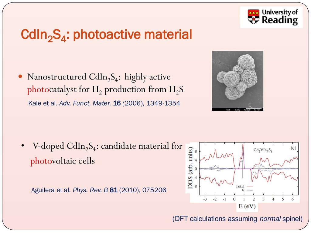
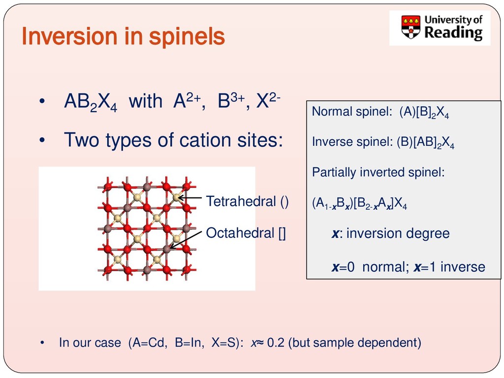
highly active photocatalyst for H2 production from H2 S Kale et al. Adv. Funct. Mater. 16 (2006), 1349-1354 • V-doped CdIn2 S4 : candidate material for photovoltaic cells Aguilera et al. Phys. Rev. B 81 (2010), 075206 (DFT calculations assuming normal spinel)
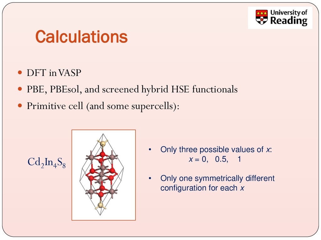
hybrid HSE functionals Primitive cell (and some supercells): Cd2 In4 S8 • Only three possible values of x: x = 0, 0.5, 1 • Only one symmetrically different configuration for each x
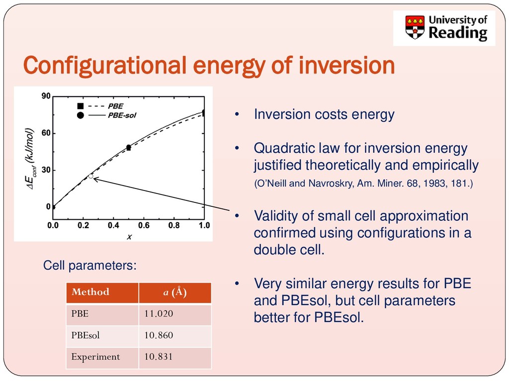
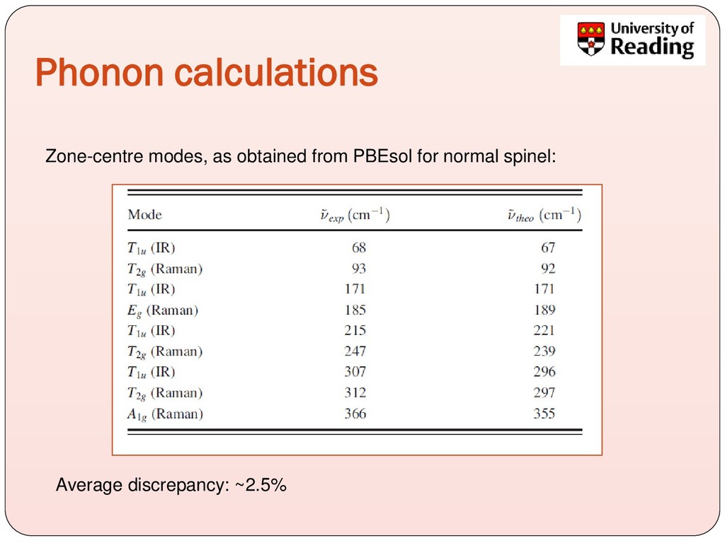
law for inversion energy justified theoretically and empirically (O’Neill and Navroskry, Am. Miner. 68, 1983, 181.) • Validity of small cell approximation confirmed using configurations in a double cell. • Very similar energy results for PBE and PBEsol, but cell parameters better for PBEsol. Method a (Å) PBE 11.020 PBEsol 10.860 Experiment 10.831 Cell parameters:
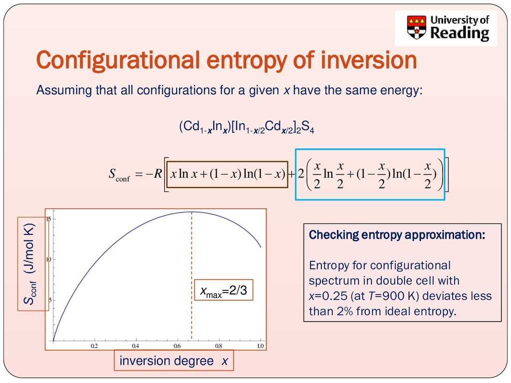
10 15 inversion degree x xmax =2/3 conf ln (1 )ln(1 ) 2 ln (1 )ln(1 ) 2 2 2 2 x x x x S R x x x x = − + − − + + − − (Cd1-x Inx )[In1-x/2 Cdx/2 ]2 S4 Assuming that all configurations for a given x have the same energy: Checking entropy approximation: Entropy for configurational spectrum in double cell with x=0.25 (at T=900 K) deviates less than 2% from ideal entropy.
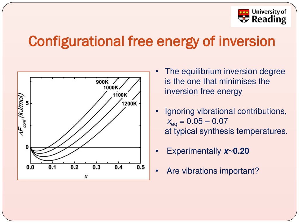
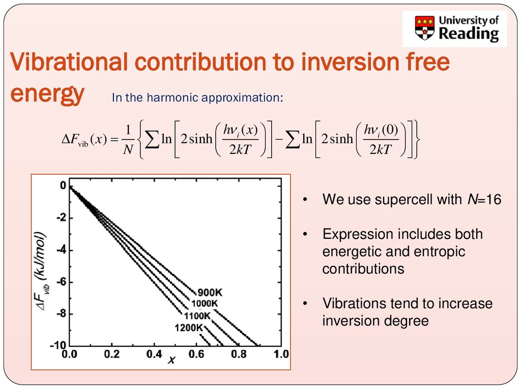
is the one that minimises the inversion free energy • Ignoring vibrational contributions, xeq = 0.05 – 0.07 at typical synthesis temperatures. • Experimentally x~0.20 • Are vibrations important?
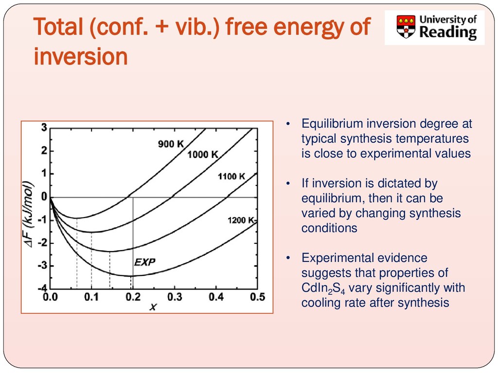
inversion degree at typical synthesis temperatures is close to experimental values • If inversion is dictated by equilibrium, then it can be varied by changing synthesis conditions • Experimental evidence suggests that properties of CdIn2 S4 vary significantly with cooling rate after synthesis
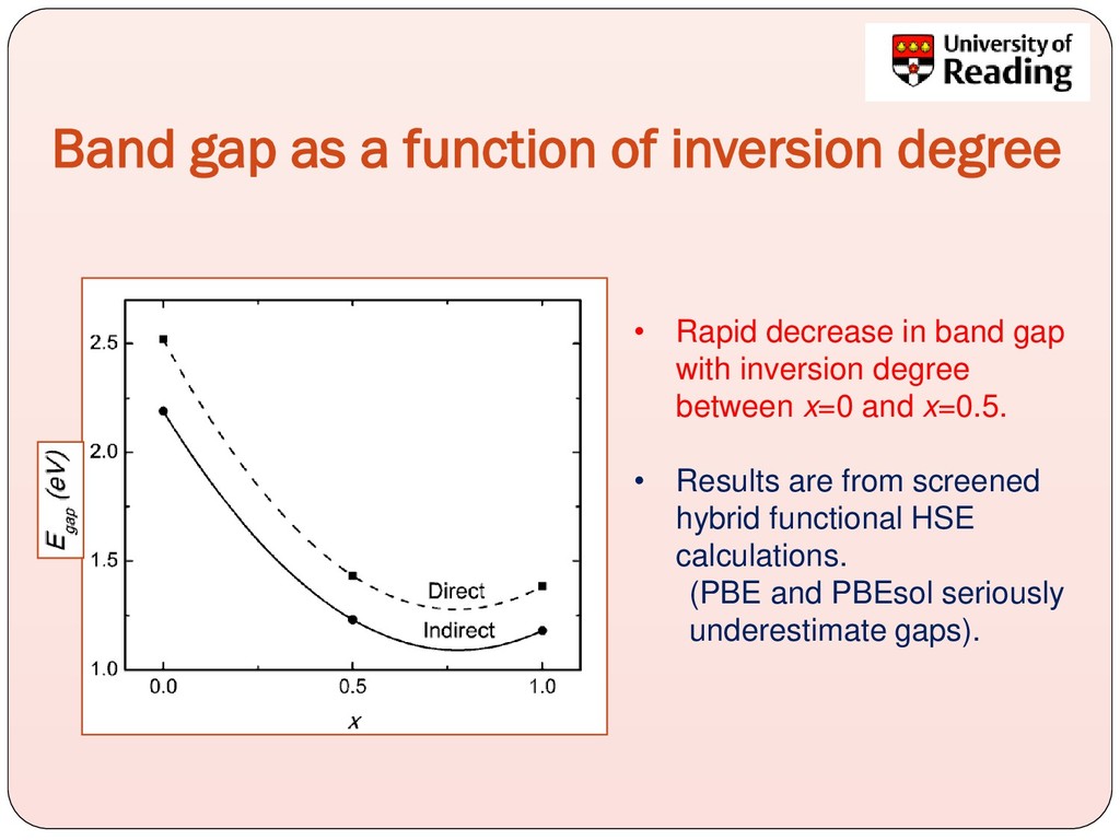
decrease in band gap with inversion degree between x=0 and x=0.5. • Results are from screened hybrid functional HSE calculations. (PBE and PBEsol seriously underestimate gaps).
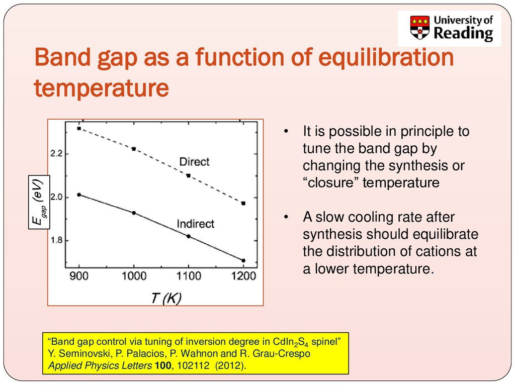
is possible in principle to tune the band gap by changing the synthesis or “closure” temperature • A slow cooling rate after synthesis should equilibrate the distribution of cations at a lower temperature. “Band gap control via tuning of inversion degree in CdIn2 S4 spinel” Y. Seminovski, P. Palacios, P. Wahnon and R. Grau-Crespo Applied Physics Letters 100, 102112 (2012).
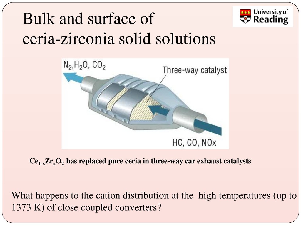
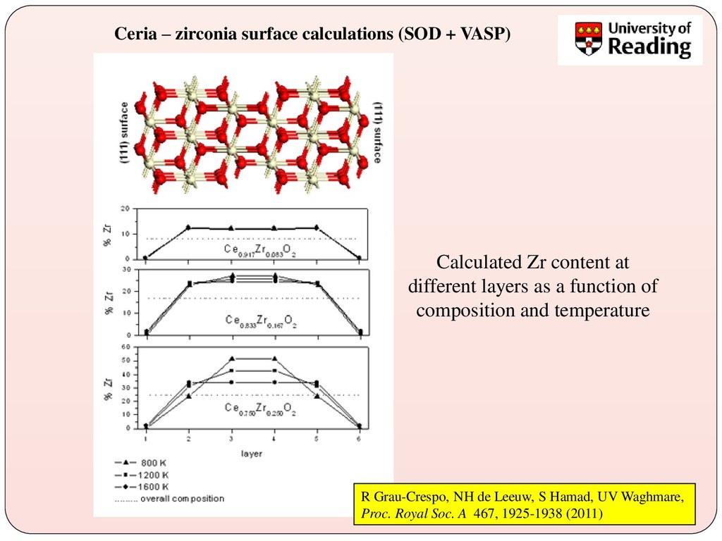
has replaced pure ceria in three-way car exhaust catalysts What happens to the cation distribution at the high temperatures (up to 1373 K) of close coupled converters?
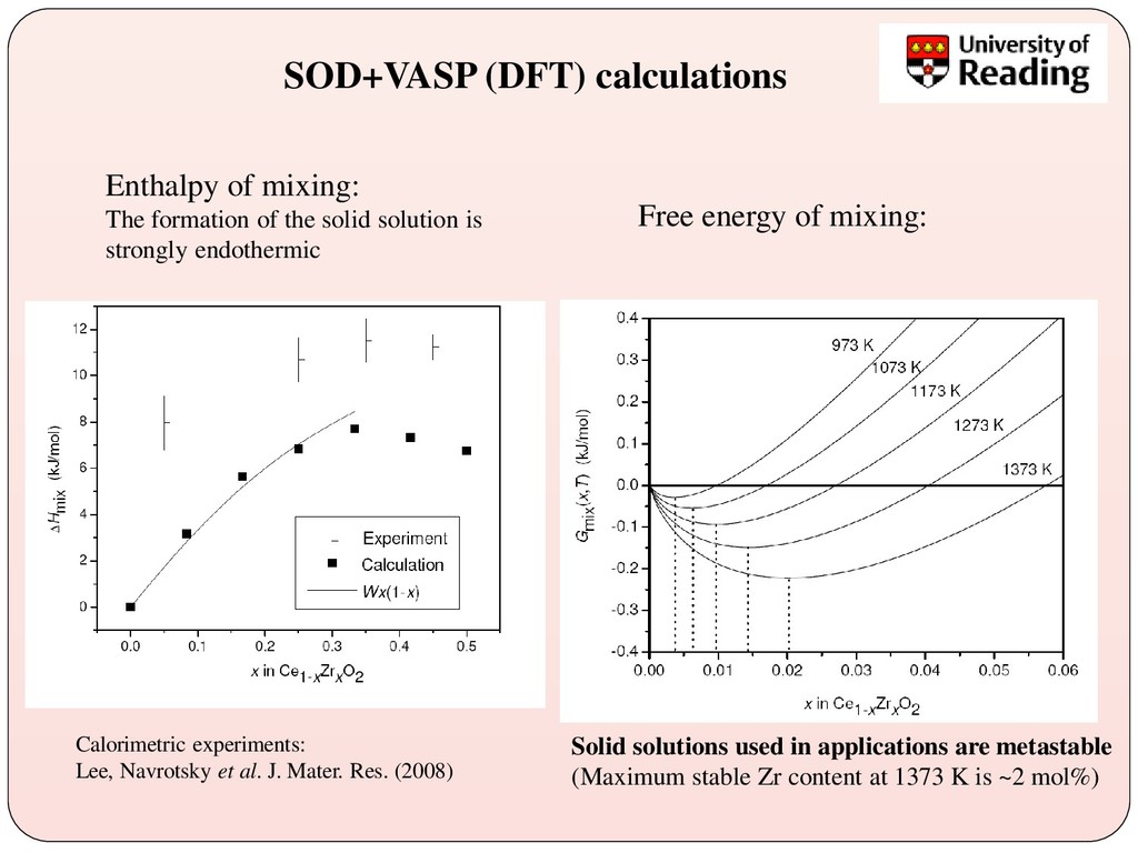
Mater. Res. (2008) Enthalpy of mixing: The formation of the solid solution is strongly endothermic Solid solutions used in applications are metastable (Maximum stable Zr content at 1373 K is ~2 mol%) Free energy of mixing:
content at different layers as a function of composition and temperature R Grau-Crespo, NH de Leeuw, S Hamad, UV Waghmare, Proc. Royal Soc. A 467, 1925-1938 (2011)
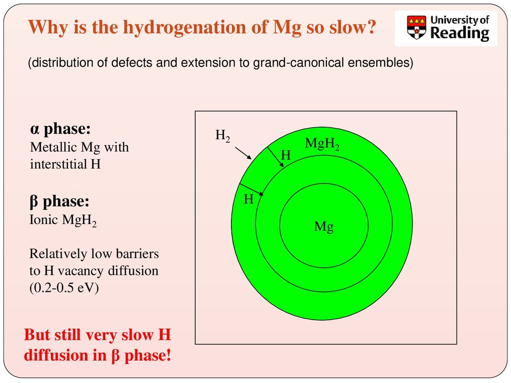
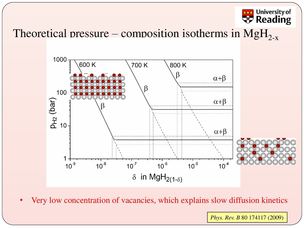
Mg Mg MgH2 H H α phase: Metallic Mg with interstitial H β phase: Ionic MgH2 But still very slow H diffusion in β phase! (distribution of defects and extension to grand-canonical ensembles) Relatively low barriers to H vacancy diffusion (0.2-0.5 eV)
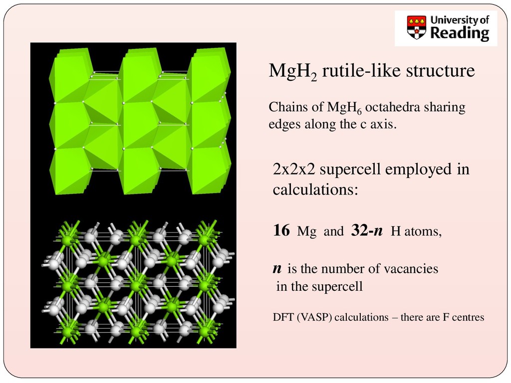
the c axis. 2x2x2 supercell employed in calculations: 16 Mg and 32-n H atoms, n is the number of vacancies in the supercell DFT (VASP) calculations – there are F centres
species: VFE(eV) 1 mono-vacancy 1.41 1+2 di-vacancy of type I 1.04 2+3 di-vacancy of type II 1.13 1+2 +3 tri-vacancy 1.07 0 1 2 3 0.0 0.1 0.2 0.3 0.4 0.5 0.6 0.7 0.8 0.9 1.0 1.1 E (eV) n (number of vacancies per supercell)
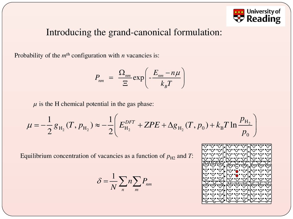
- nm nm nm B E n P k T − = µ is the H chemical potential in the gas phase: 2 2 2 2 2 H H H H H 0 B 0 1 1 ( , ) ( , ) ln 2 2 DFT p g T p E ZPE g T p k T p = − − + + + 1 nm n m n P N = Equilibrium concentration of vacancies as a function of pH2 and T: Introducing the grand-canonical formulation:
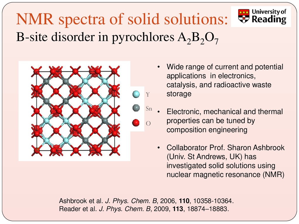
B2 O7 Y Sn O • Wide range of current and potential applications in electronics, catalysis, and radioactive waste storage • Electronic, mechanical and thermal properties can be tuned by composition engineering • Collaborator Prof. Sharon Ashbrook (Univ. St Andrews, UK) has investigated solid solutions using nuclear magnetic resonance (NMR) Ashbrook et al. J. Phys. Chem. B, 2006, 110, 10358-10364. Reader et al. J. Phys. Chem. B, 2009, 113, 18874–18883.
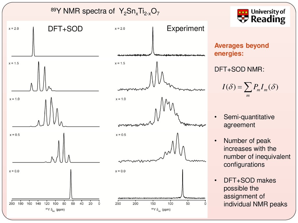
Averages beyond energies: DFT+SOD NMR: • Semi-quantitative agreement • Number of peak increases with the number of inequivalent configurations • DFT+SOD makes possible the assignment of individual NMR peaks ( ) ( ) m m m I P I =
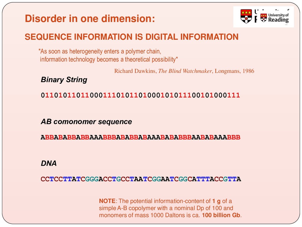
a polymer chain, information technology becomes a theoretical possibility" Richard Dawkins, The Blind Watchmaker, Longmans, 1986 Binary String 011010110110001110101101000101011100101000111 AB comonomer sequence ABBABABBABBAAABBBABABBABAAABABABBBAABABAAABBB DNA CCTCCTTATCGGGACCTGCCTAATCGGAATCGGCATTTACCGTTA NOTE: The potential information-content of 1 g of a simple A-B copolymer with a nominal Dp of 100 and monomers of mass 1000 Daltons is ca. 100 billion Gb. Disorder in one dimension:
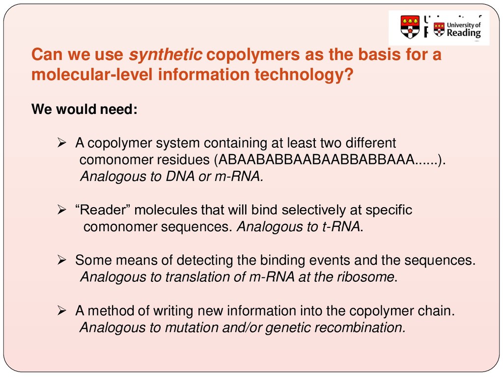
molecular-level information technology? We would need: ➢ A copolymer system containing at least two different comonomer residues (ABAABABBAABAABBABBAAA......). Analogous to DNA or m-RNA. ➢ “Reader” molecules that will bind selectively at specific comonomer sequences. Analogous to t-RNA. ➢ Some means of detecting the binding events and the sequences. Analogous to translation of m-RNA at the ribosome. ➢ A method of writing new information into the copolymer chain. Analogous to mutation and/or genetic recombination.
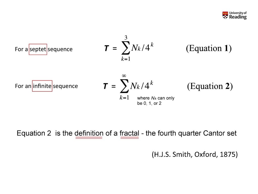
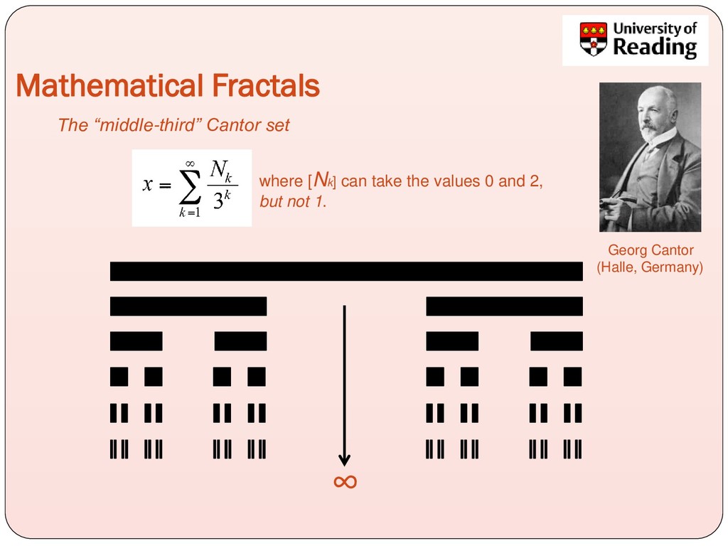
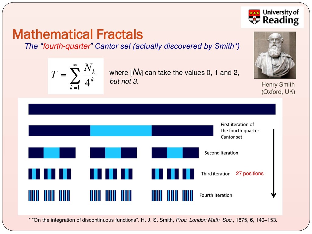
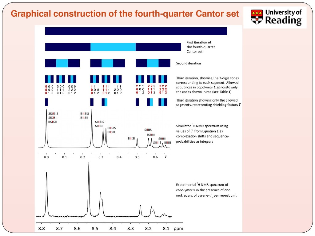
∞ Henry Smith (Oxford, UK) where [Nk] can take the values 0, 1 and 2, but not 3. (27 positions) * “On the integration of discontinuous functions”. H. J. S. Smith, Proc. London Math. Soc., 1875, 6, 140–153.
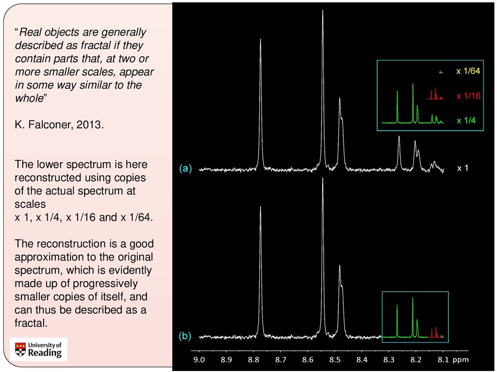
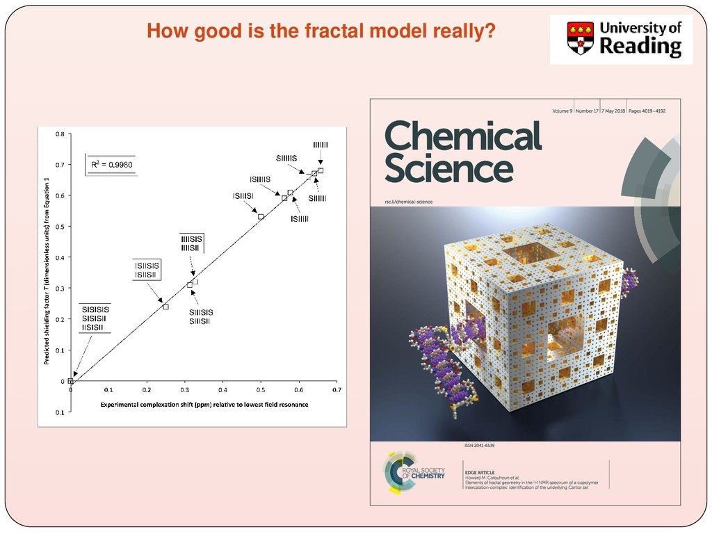
parts that, at two or more smaller scales, appear in some way similar to the whole” K. Falconer, 2013. The lower spectrum is here reconstructed using copies of the actual spectrum at scales x 1, x 1/4, x 1/16 and x 1/64. The reconstruction is a good approximation to the original spectrum, which is evidently made up of progressively smaller copies of itself, and can thus be described as a fractal.
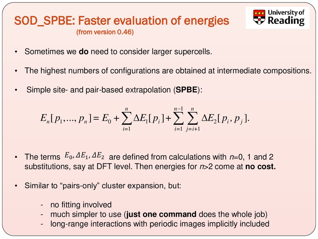
we do need to consider larger supercells. • The highest numbers of configurations are obtained at intermediate compositions. • Simple site- and pair-based extrapolation (SPBE): • The terms are defined from calculations with n=0, 1 and 2 substitutions, say at DFT level. Then energies for n>2 come at no cost. • Similar to “pairs-only” cluster expansion, but: - no fitting involved - much simpler to use (just one command does the whole job) - long-range interactions with periodic images implicitly included 1 1 0 1 2 1 1 1 [ ,..., ] [ ] [ ]. n n n n n i i j i= i= j=i+ E p p = E + E p + E p , p − 0 , 1 , 2
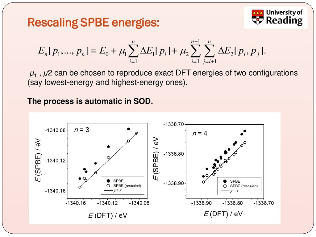
1 1 1 [ ,..., ] [ ] [ ]. n n n n n i i j i= i= j=i+ E p p = E + E p + E p , p − μ1 , μ2 can be chosen to reproduce exact DFT energies of two configurations (say lowest-energy and highest-energy ones). The process is automatic in SOD.
Thornstrom - Victor Posligua - Scott Midgley Collaborators - Dr. Said Hamad (UPO, Seville) - Prof. Nora de Leeuw (Cardiff) - Prof. Richard Catlow (UCL / Cardiff) - Dr. Rabdel Ruiz-Salvador (UPO Seville) - Dr Norge Cruz-Hernandez (Seville) - Prof. Umesh Waghmare (JNCASR, India) - Dr Kyle Smith (Purdue, US) - Prof. Tim Fisher (Purdue, US) - Dr Yohanna Seminovski - Prof. Perla Wahnon (UPM, Madrid) - Prof. Sharon Ashbrook (St Andrews, UK) - Howard Colquhoun (Reading) UK Materials Chemistry Consortium and for access to the National Supercomputing Facilities (ARCHER).
![Ricardo Grau-Crespo [email protected] Department of Chemistry University of Reading United](https://files.speakerdeck.com/presentations/6a3a882c20b24d8598cc66ab317160c3/slide_0.jpg)