function •Degrees of freedom •“Sampling” as source of all uncertainty •Defining random effects via sampling design •Neglect of data uncertainty •add your own
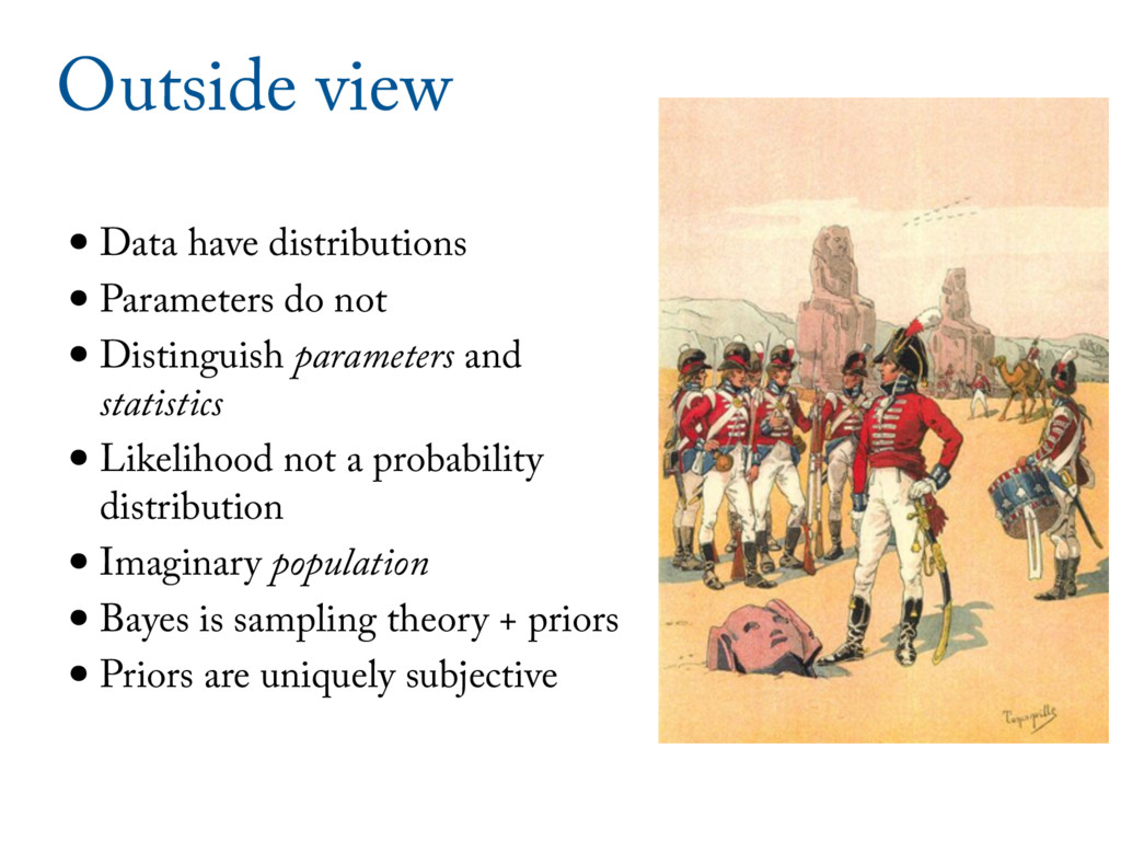
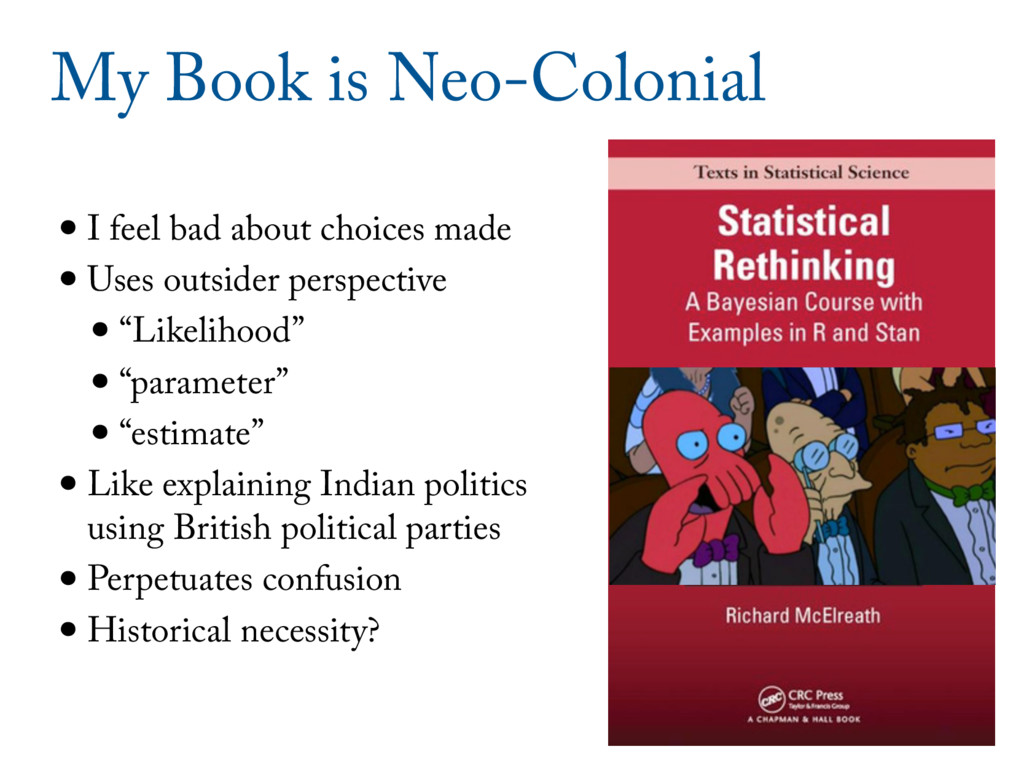
•Uses outsider perspective •“Likelihood” •“parameter” •“estimate” •Like explaining Indian politics using British political parties •Perpetuates confusion •Historical necessity?
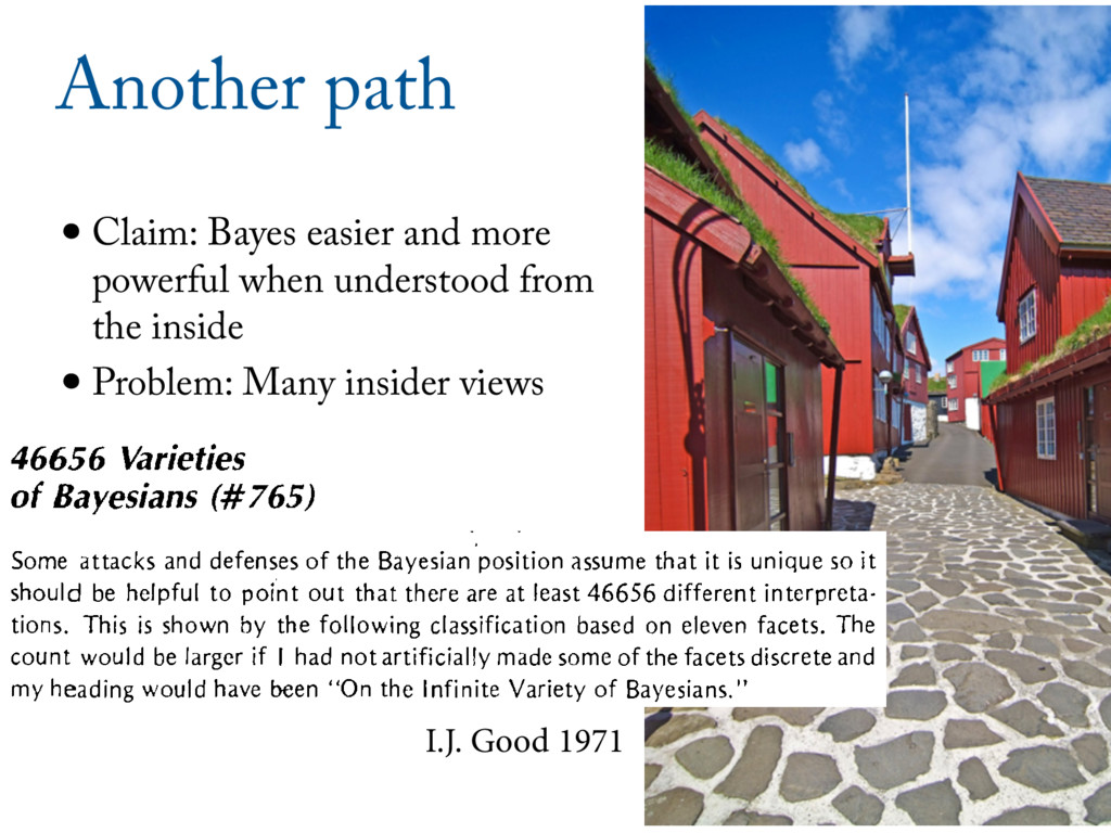
from the inside •Problem: Many insider views CHAPTER 3 46656 Varieties of Bayesians (#765) . . Some attacks and defenses of the ~a~esian'~osition assume that i t is unique so i t should be helpful to point out that there are at least 46656 different interpreta- tions. This is shown by the following classification based on eleven facets. The count would be larger i f I had not artificially made some of the facets discrete and my heading would have been "On the Infinite Variety of Bayesians." All Bayesians, as I understand the term, believe that it is usually meaningful to talk about the probability of a hypothesis and they make some attempt to be con- sistent in their judgments. Thus von Mises (1942) would not count as a Bayesian, tions; ( tive pro Hegel a after th 5. U (c) utilit 6. Q nition t informa using q use of q think th 7. P exist bu 8. I credibil think o that cre nationa 9. D imagina from wh see ##13 10. A (comple venient 46656 V A R I E T CHAPTER 3 46656 Varieties of Bayesians (#765) . . Some attacks and defenses of the ~a~esian'~osition assume that i t is unique so i t should be helpful to point out that there are at least 46656 different interpreta- tions. This is shown by the following classification based on eleven facets. The count would be larger i f I had not artificially made some of the facets discrete and my heading would have been "On the Infinite Variety of Bayesians." All Bayesians, as I understand the term, believe that it is usually meaningful to talk about the probability of a hypothesis and they make some attempt to be con- sistent in their judgments. Thus von Mises (1942) would not count as a Bayesian, 4. Extremeness. (a) Formal Bayesian procedu tions; (b) non-Bayesian methods used provided t tive probability are not seen to be contradicted (th Hegel and Marx would call i t a synthesis); (c) n after they have been given a rough Bayesian justif 5. Utilities. (a) Brought in from the start; (c) utilities introduced separately from intuitive p 6. Quasiutilities. (a) Only one kind of utility nition that "quasiutilities" (#%90A, 755) are w information or "weights of evidence" (Peirce, 1 using quasiutilities without noticing that they use of quasiutilities is as old as the words "infor think the name "quasiutility" serves a useful purp 7. Physical probabilities. (a) Assumed to exis exist but without philosophical commitment (#6 8. Intuitive probability. (a) Subjective proba credibilities (logical probabilities) primary; (c) reg think of subjective probabilities as estimates of that credibilities really exist; (d) credibilities in national body. . . . 9. Device of imaginary results. (a) Explicit u imaginary experimental results used for judging from which are inferred discernments about the in see ##13, 547. 10. Axioms. (a) As simple as possible; (b) inc (complete additivity); (c) using Kolmogorov's ax I.J. Good 1971
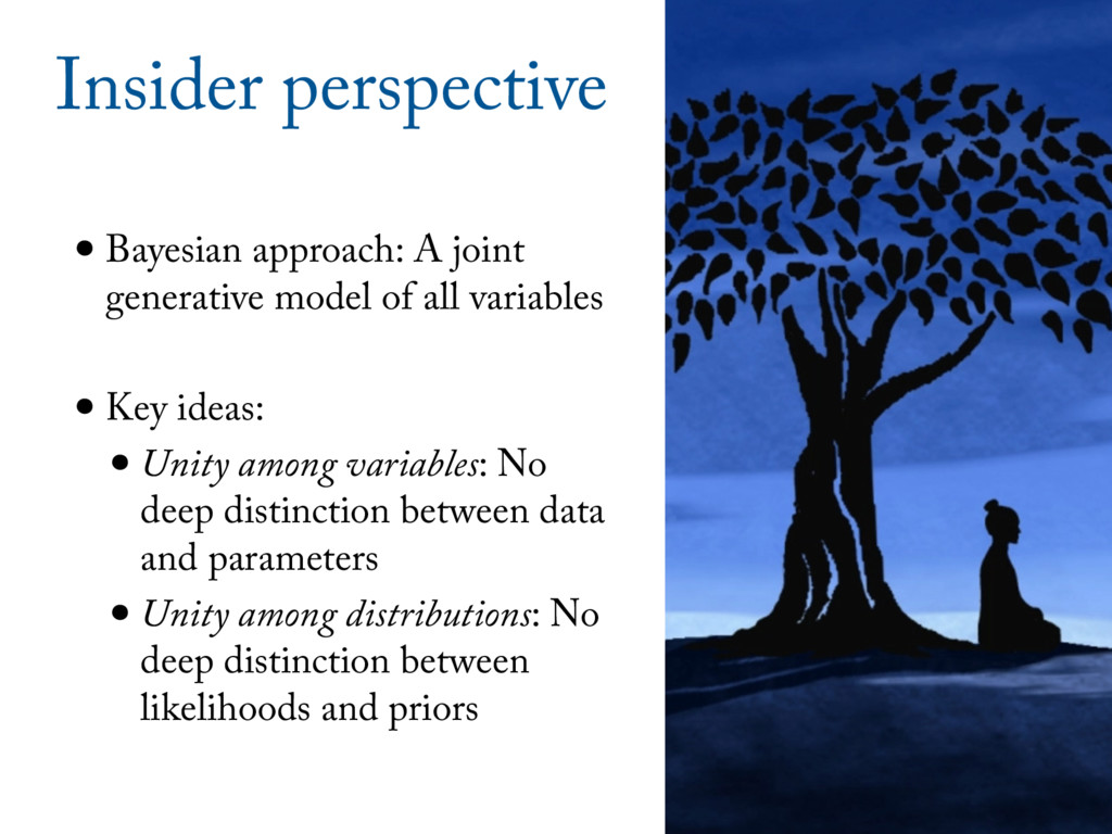
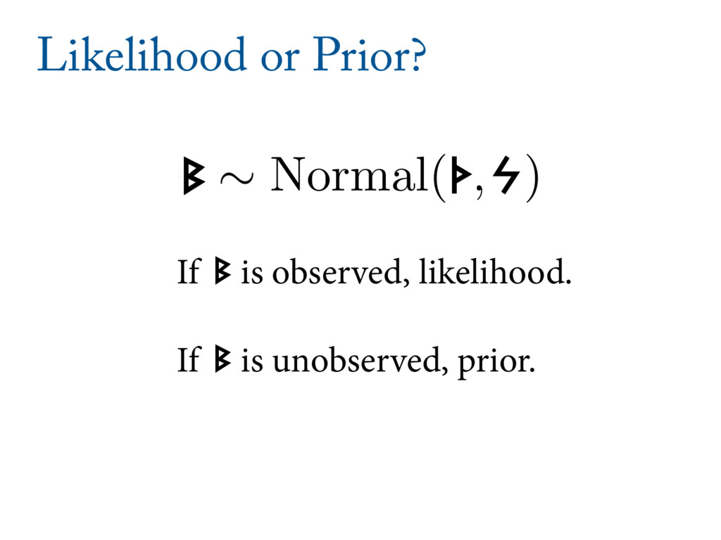
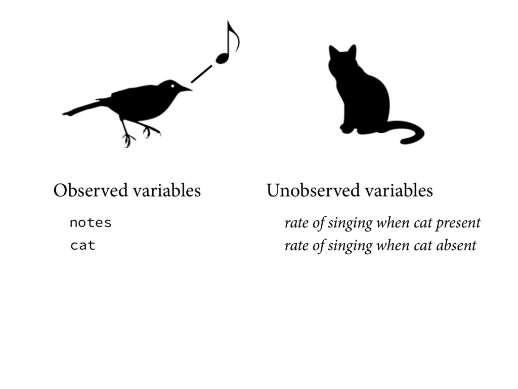
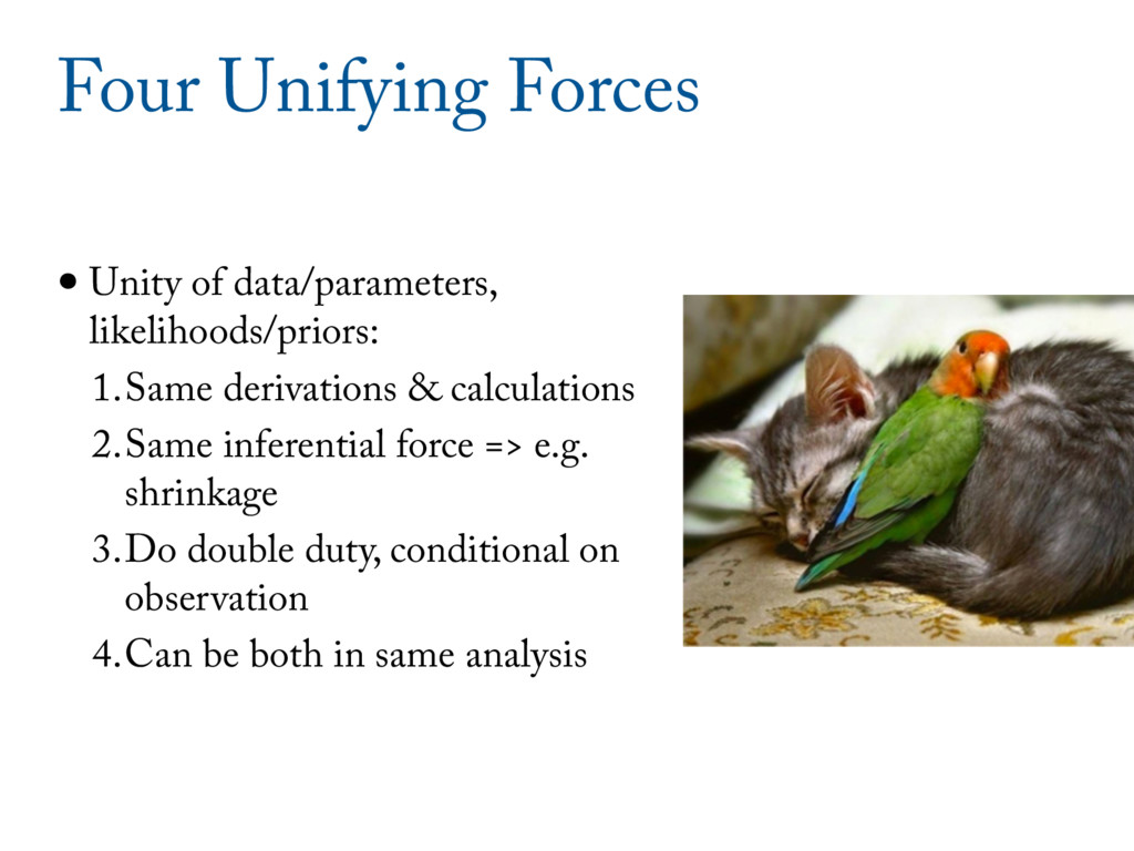
variables •Key ideas: •Unity among variables: No deep distinction between data and parameters •Unity among distributions: No deep distinction between likelihoods and priors
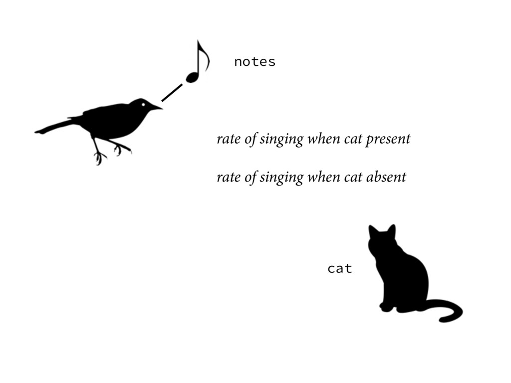
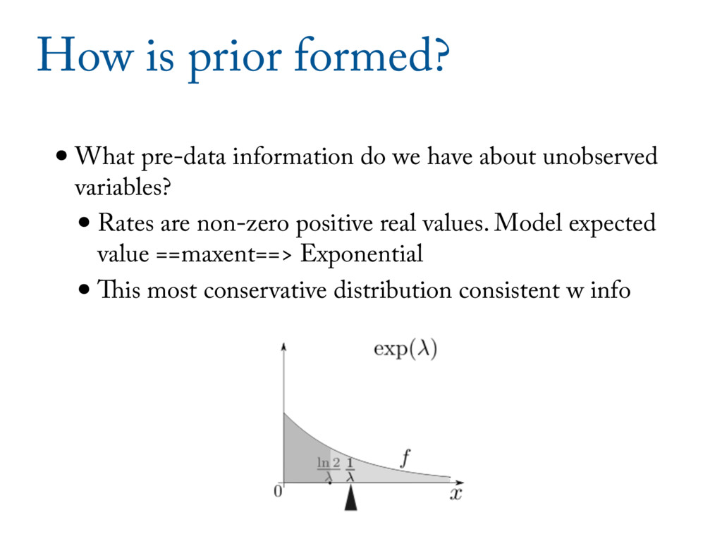
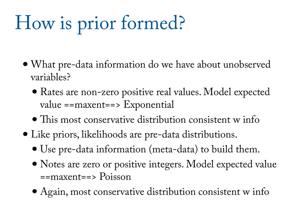
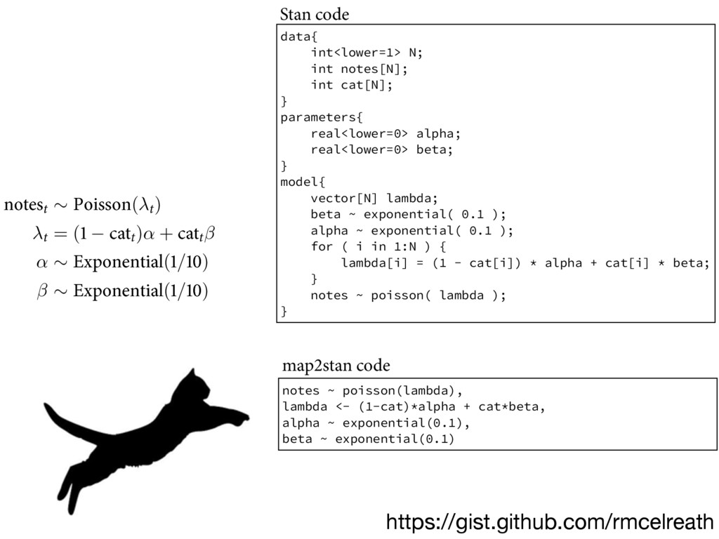
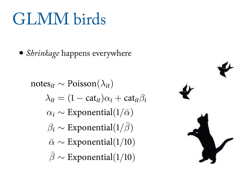
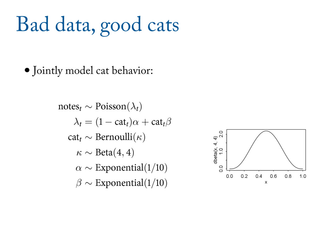
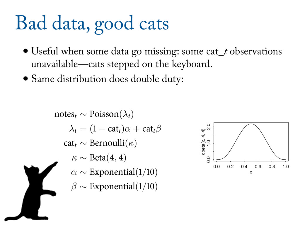
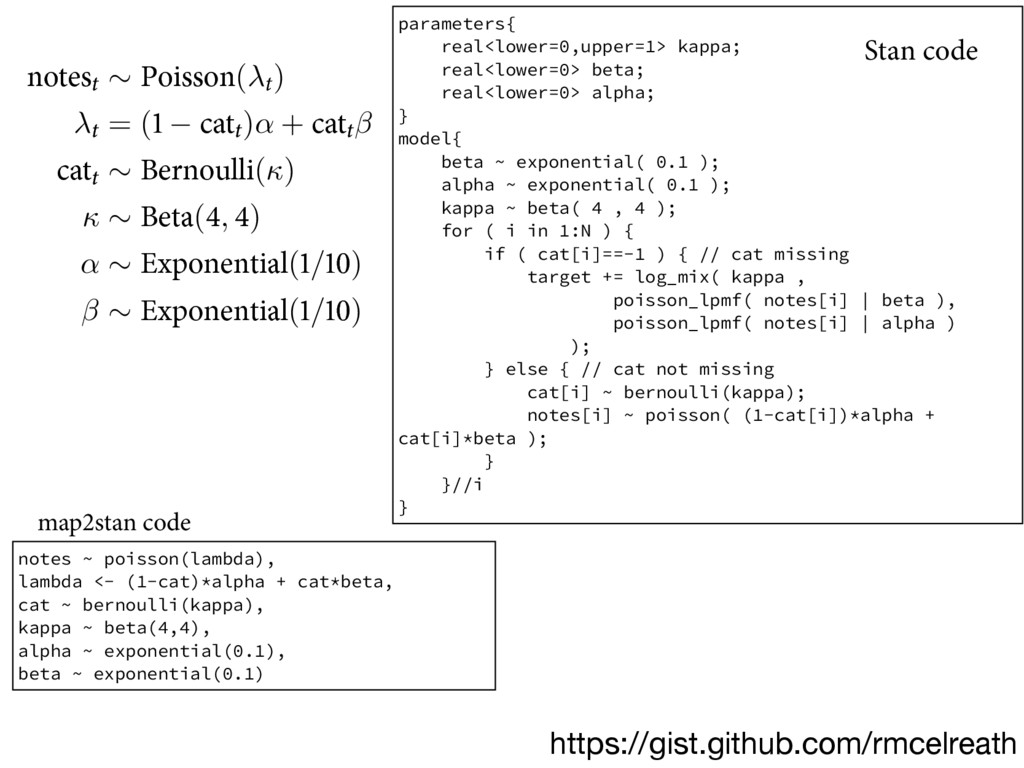
about unobserved variables? •Rates are non-zero positive real values. Model expected value ==maxent==> Exponential •This most conservative distribution consistent w info •Like priors, likelihoods are pre-data distributions. •Use pre-data information (meta-data) to build them. •Notes are zero or positive integers. Model expected value ==maxent==> Poisson •Again, most conservative distribution consistent w info
about unobserved variables? •Rates are non-zero positive real values. Model expected value ==maxent==> Exponential •This most conservative distribution consistent w info •Like priors, likelihoods are pre-data distributions. •Use pre-data information (meta-data) to build them. •Notes are zero or positive integers. Model expected value ==maxent==> Poisson •Again, most conservative distribution consistent w info
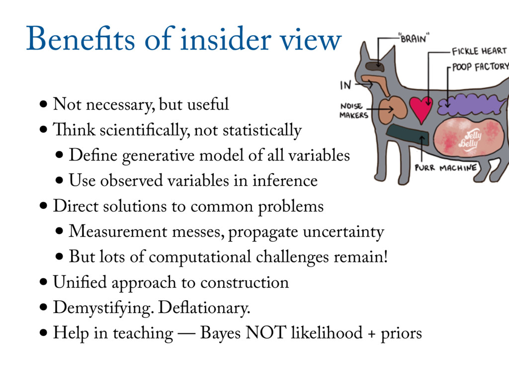
not statistically •Define generative model of all variables •Use observed variables in inference •Direct solutions to common problems •Measurement messes, propagate uncertainty •But lots of computational challenges remain! •Unified approach to construction •Demystifying. Deflationary. •Help in teaching — Bayes NOT likelihood + priors
![data{ int<lower=1> N; int<lower=1> N_id; int notes[N]; int cat[N]; int](https://files.speakerdeck.com/presentations/faee2244beca472fa35b8e2a66c83d1e/slide_28.jpg)
![generated quantities{ vector[N] cat_impute; for ( i in 1:N )](https://files.speakerdeck.com/presentations/faee2244beca472fa35b8e2a66c83d1e/slide_32.jpg)