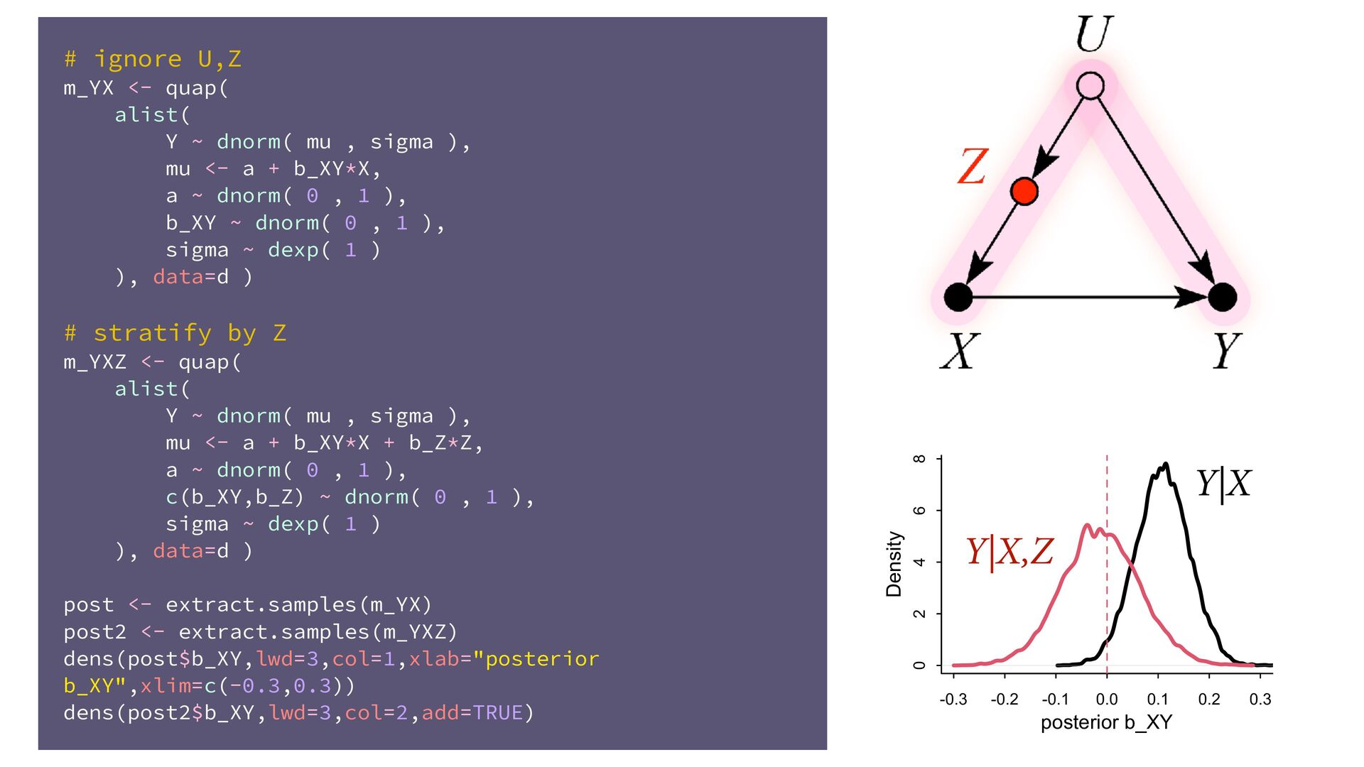
mu , sigma ), mu <- a + b_XY*X, a ~ dnorm( 0 , 1 ), b_XY ~ dnorm( 0 , 1 ), sigma ~ dexp( 1 ) ), data=d ) # stratify by Z m_YXZ <- quap( alist( Y ~ dnorm( mu , sigma ), mu <- a + b_XY*X + b_Z*Z, a ~ dnorm( 0 , 1 ), c(b_XY,b_Z) ~ dnorm( 0 , 1 ), sigma ~ dexp( 1 ) ), data=d ) post <- extract.samples(m_YX) post2 <- extract.samples(m_YXZ) dens(post$b_XY,lwd=3,col=1,xlab="posterior b_XY",xlim=c(-0.3,0.3)) dens(post2$b_XY,lwd=3,col=2,add=TRUE) Y|X,Z Y|X -0.3 -0.2 -0.1 0.0 0.1 0.2 0.3 0 2 4 6 8 posterior b_XY Density