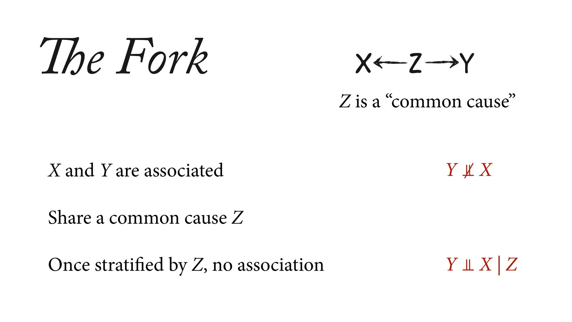
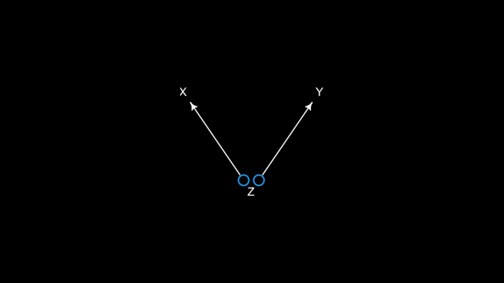
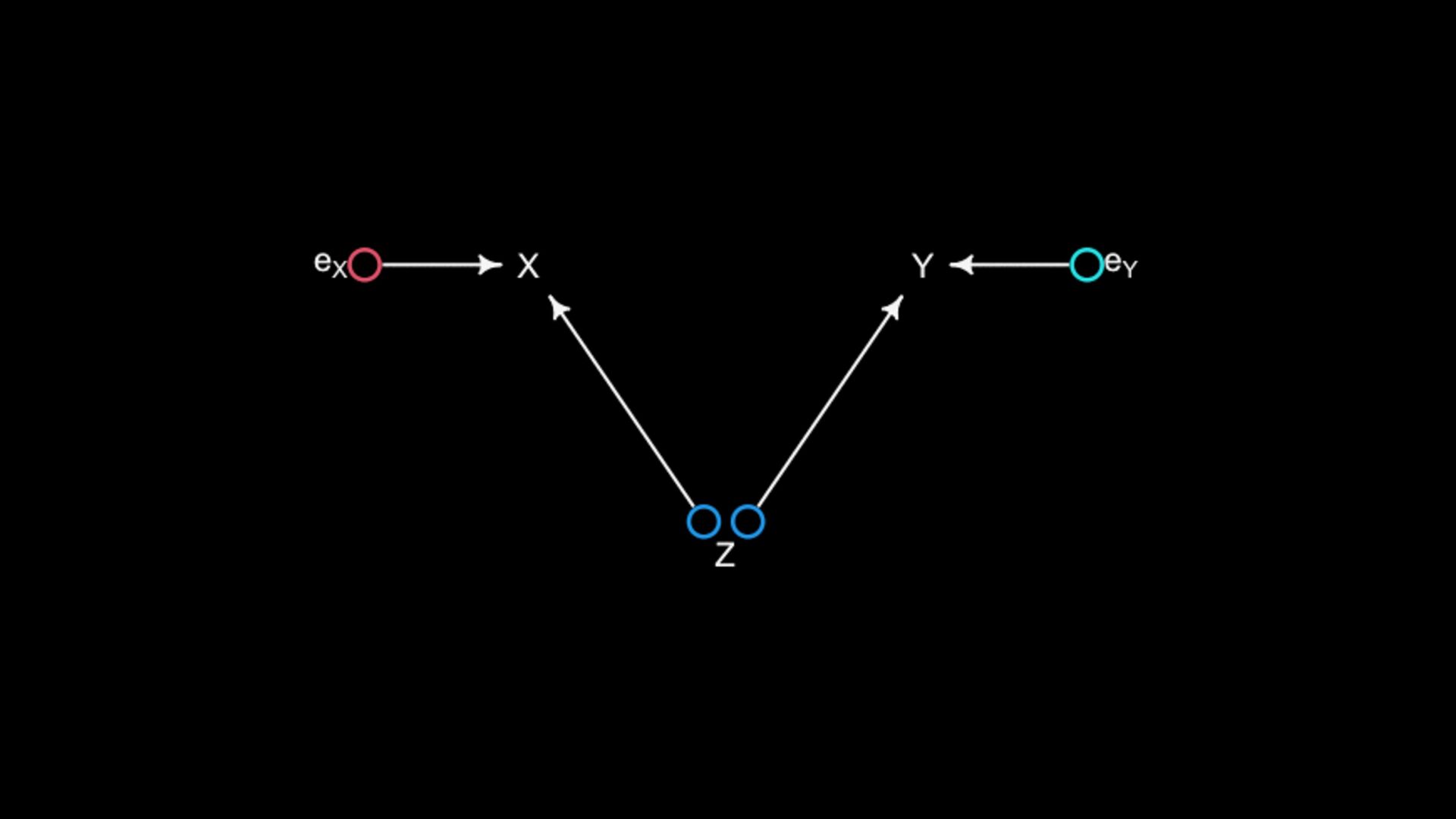
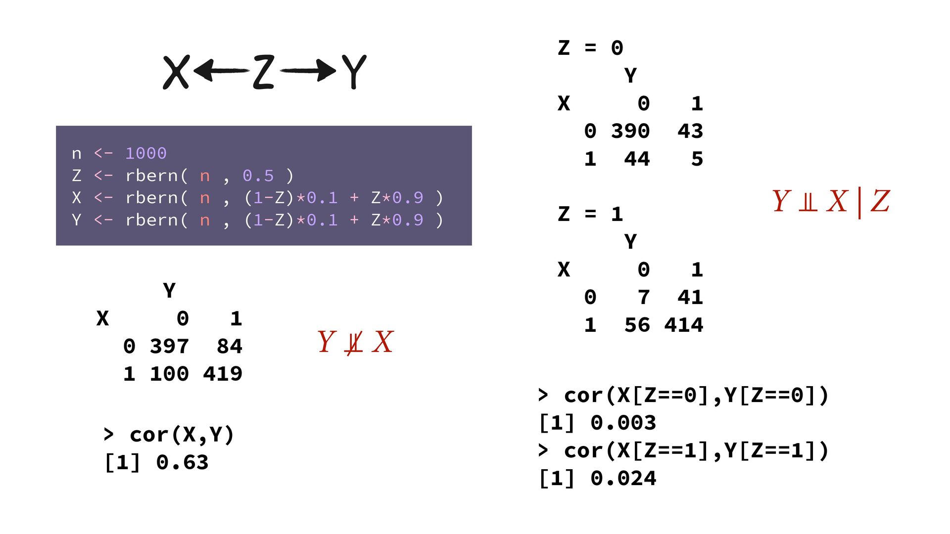
Z = 0 Y X 0 1 0 390 43 1 44 5 Z = 1 Y X 0 1 0 7 41 1 56 414 X Z Y n <- 1000 Z <- rbern( n , 0.5 ) X <- rbern( n , (1-Z)*0.1 + Z*0.9 ) Y <- rbern( n , (1-Z)*0.1 + Z*0.9 ) > cor(X,Y) [1] 0.63 > cor(X[Z==0],Y[Z==0]) [1] 0.003 > cor(X[Z==1],Y[Z==1]) [1] 0.024 Y ⫫ X Y ⫫ X | Z
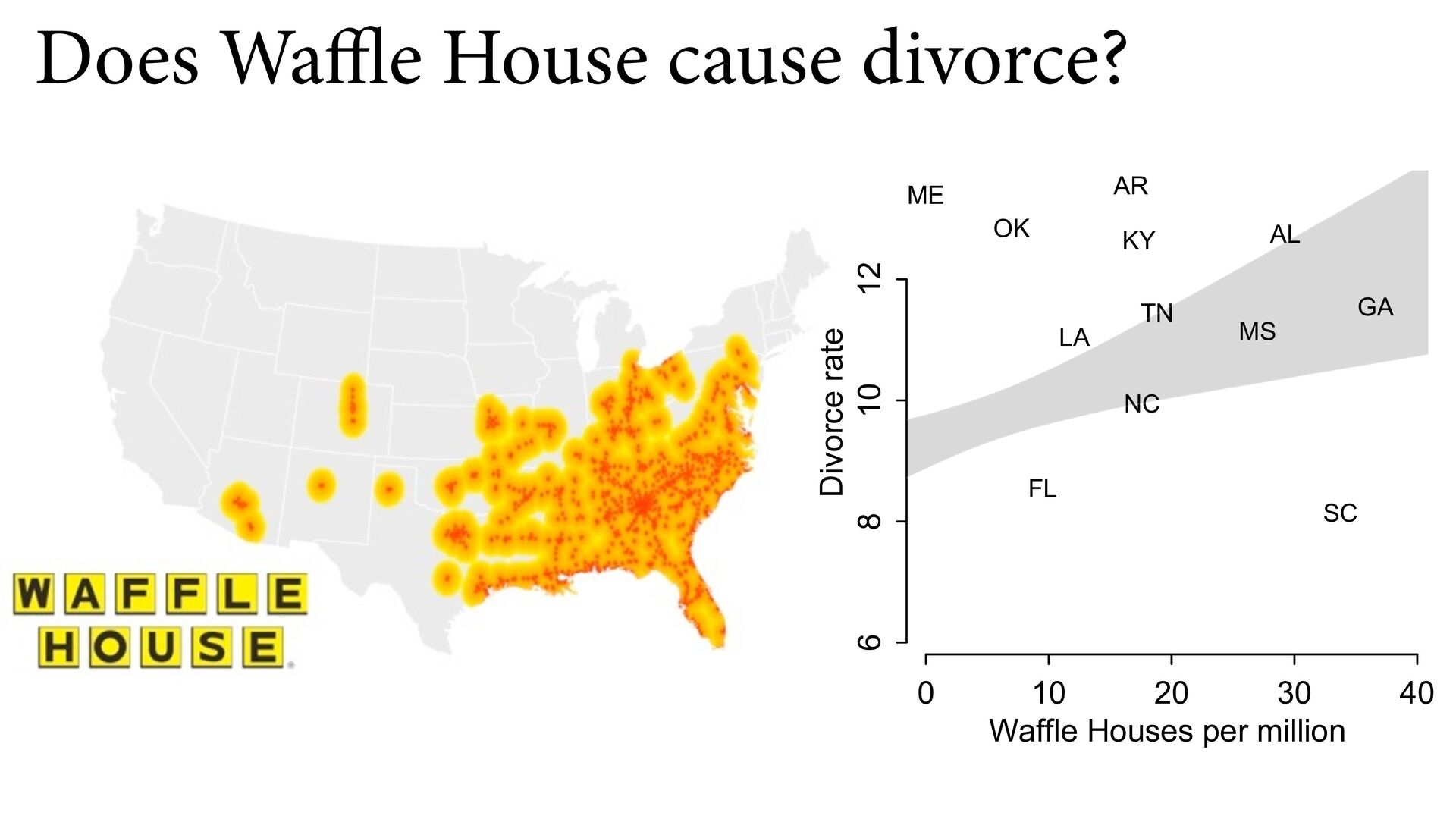
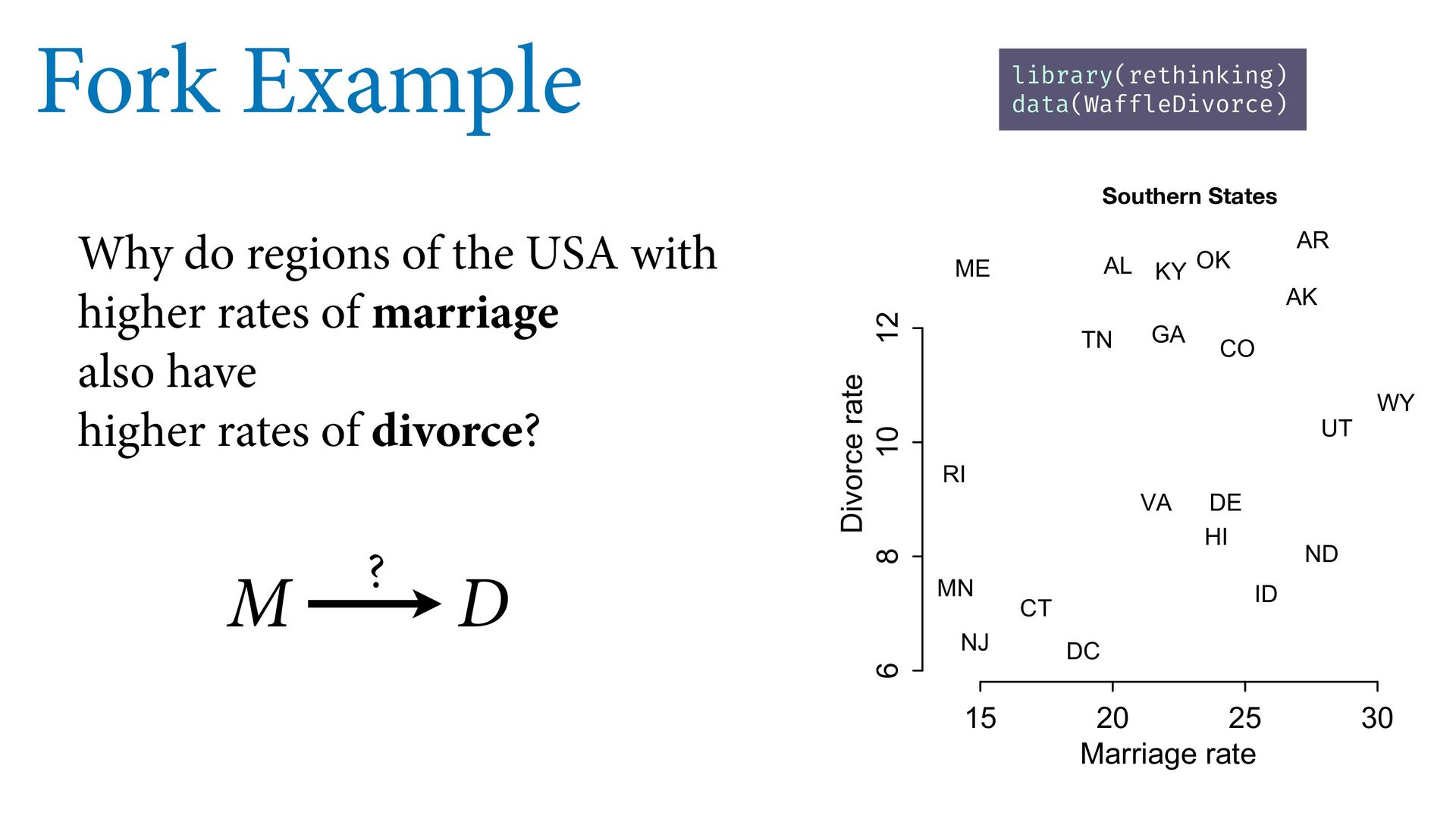
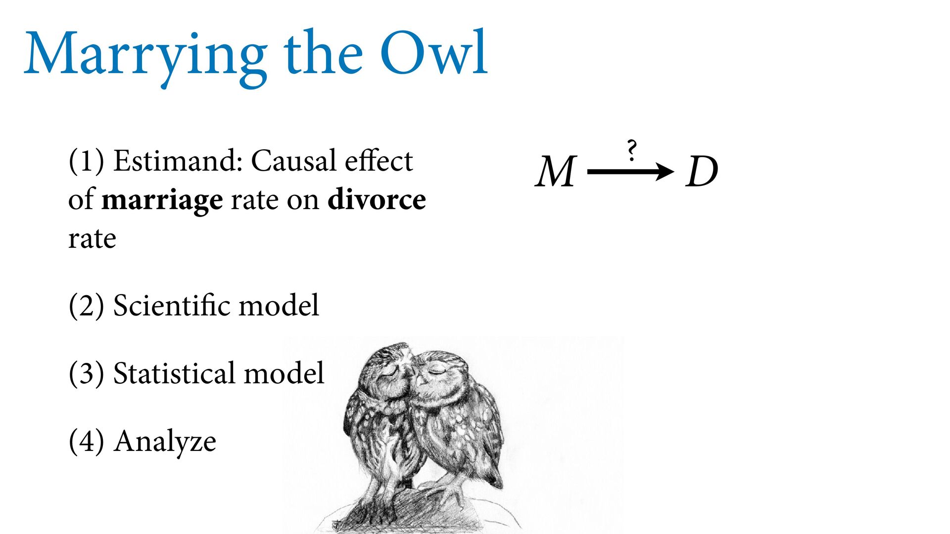
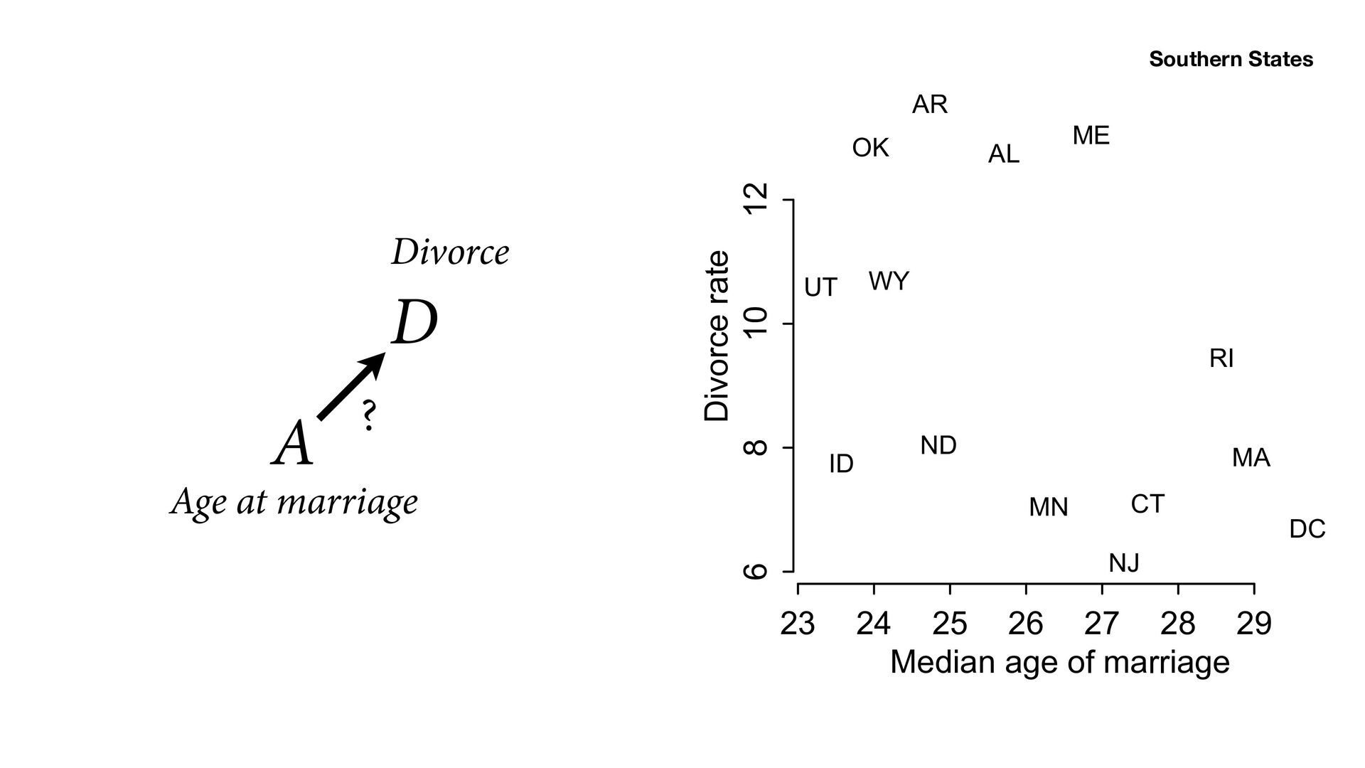
higher rates of marriage also have higher rates of divorce? 15 20 25 30 6 8 10 12 Marriage rate Divorce rate AL AK AR CO CT DE DC GA HI ID KY ME MN NJ ND OK RI TN UT VA WY library(rethinking) data(WaffleDivorce) M D ? 15 20 25 30 6 8 10 12 Marriage rate Divorce rate AL AK AR CO CT DE DC GA HI ID KY ME MN NJ ND OK RI TN UT VA WY Southern States
26 27 28 29 6 8 10 12 Median age of marriage Divorce rate AL AR CT DC ID ME MA MN NJ ND OK RI UT WY 15 20 25 30 6 8 10 12 Marriage rate Divorce rate AL AK AR CO CT DE DC GA HI ID KY ME MN NJ ND OK RI TN UT VA WY Southern States
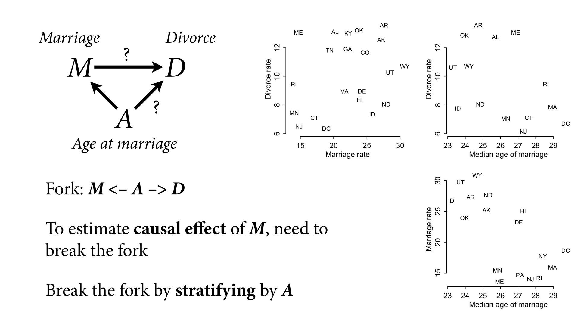
Divorce rate AL AK AR CO CT DE DC GA HI ID KY ME MN NJ ND OK RI TN UT VA WY M D A Age at marriage ? Marriage Divorce 23 24 25 26 27 28 29 6 8 10 12 Median age of marriage Divorce rate AL AR CT DC ID ME MA MN NJ ND OK RI UT WY 23 24 25 26 27 28 29 15 20 25 30 Median age of marriage Marriage rate AK AR DE DC HI ID ME MA MN NJ NY ND OK PA RI UT WY ?
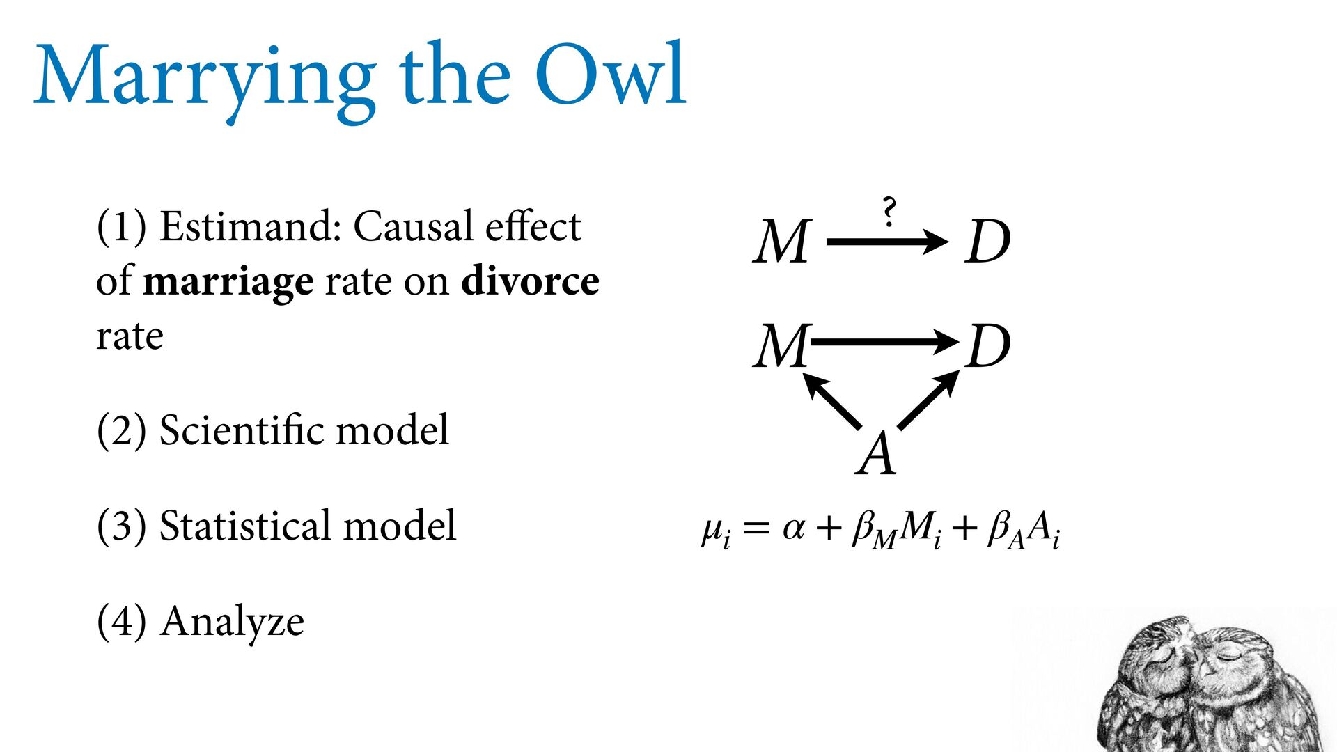
Divorce rate AL AK AR CO CT DE DC GA HI ID KY ME MN NJ ND OK RI TN UT VA WY M D A Age at marriage ? Marriage Divorce 23 24 25 26 27 28 29 6 8 10 12 Median age of marriage Divorce rate AL AR CT DC ID ME MA MN NJ ND OK RI UT WY 23 24 25 26 27 28 29 15 20 25 30 Median age of marriage Marriage rate AK AR DE DC HI ID ME MA MN NJ NY ND OK PA RI UT WY ? Fork: M <– A –> D To estimate causal effect of M, need to break the fork Break the fork by stratifying by A
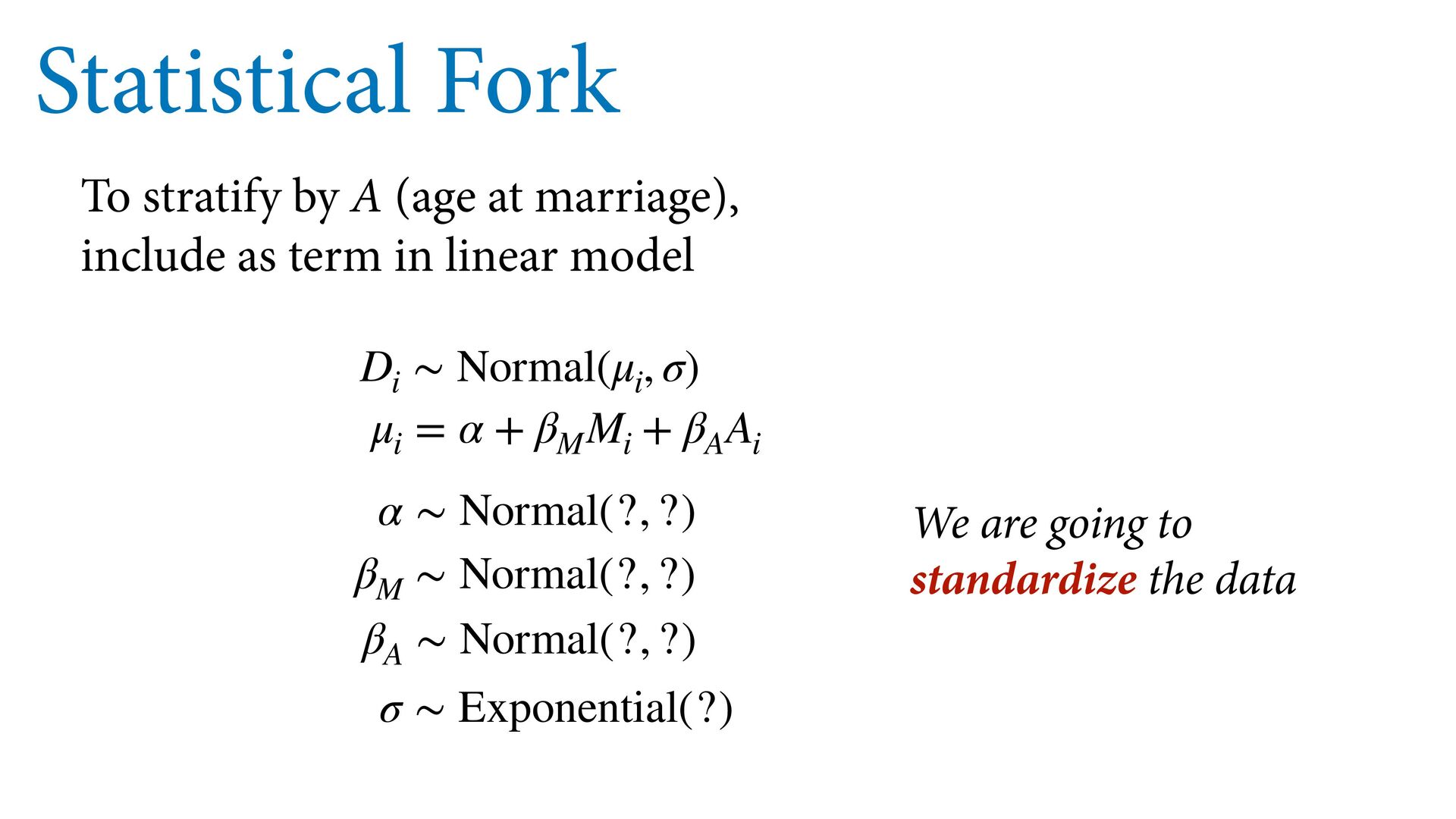
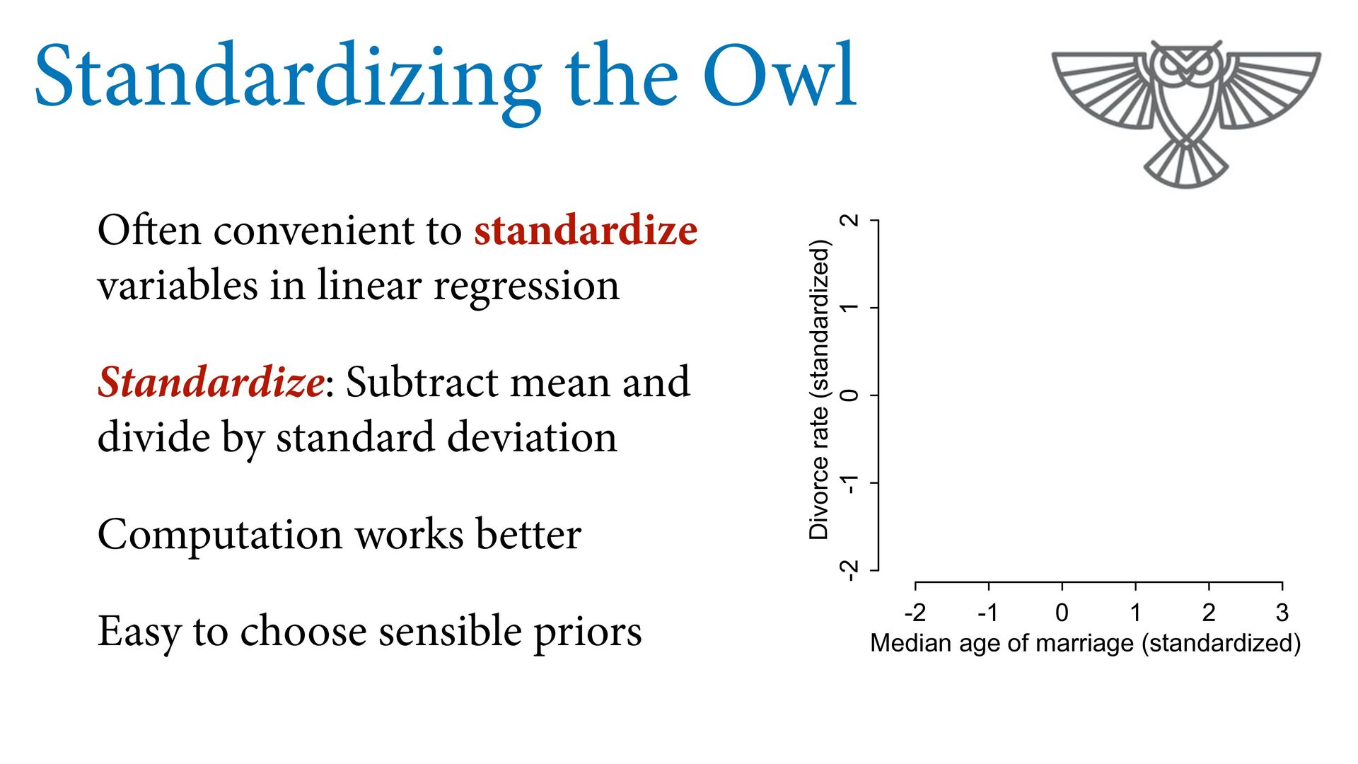
as term in linear model μ i = α + β M M i + β A A i D i ∼ Normal(μ i , σ) α ∼ Normal(?, ?) β M ∼ Normal(?, ?) β A ∼ Normal(?, ?) σ ∼ Exponential(?) We are going to standardize the data
regression Standardize: Subtract mean and divide by standard deviation Computation works better Easy to choose sensible priors -2 -1 0 1 2 3 -2 -1 0 1 2 Median age of marriage (standardized) Divorce rate (standardized)
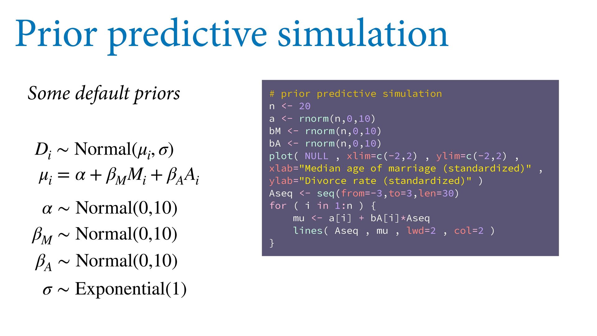
M i + β A A i D i ∼ Normal(μ i , σ) α ∼ Normal(0,10) β M ∼ Normal(0,10) β A ∼ Normal(0,10) σ ∼ Exponential(1) Some default priors # prior predictive simulation n <- 20 a <- rnorm(n,0,10) bM <- rnorm(n,0,10) bA <- rnorm(n,0,10) plot( NULL , xlim=c(-2,2) , ylim=c(-2,2) , xlab="Median age of marriage (standardized)" , ylab="Divorce rate (standardized)" ) Aseq <- seq(from=-3,to=3,len=30) for ( i in 1:n ) { mu <- a[i] + bA[i]*Aseq lines( Aseq , mu , lwd=2 , col=2 ) }
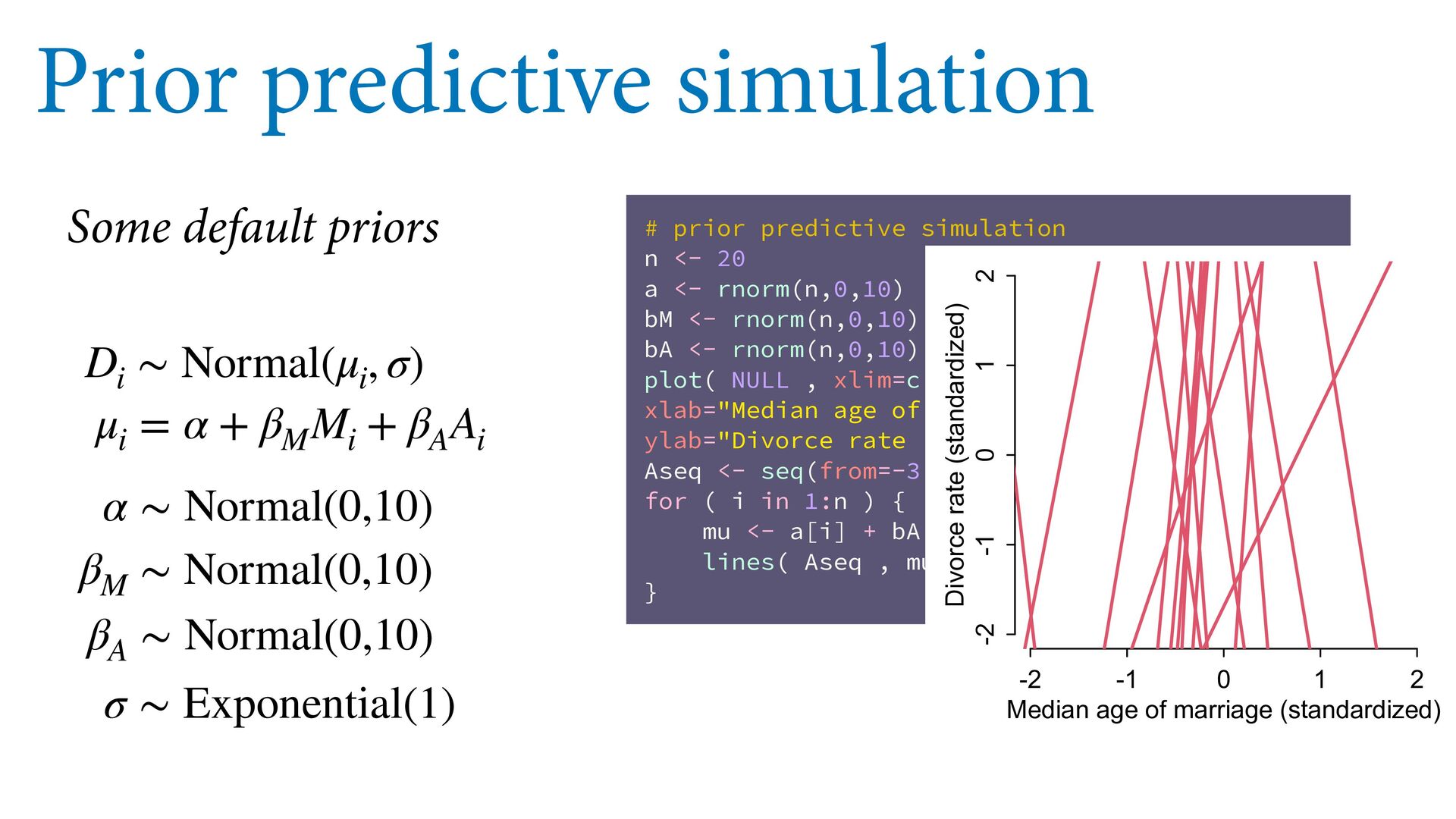
bM <- rnorm(n,0,10) bA <- rnorm(n,0,10) plot( NULL , xlim=c(-2,2) , ylim=c(-2,2) , xlab="Median age of marriage (standardized)" , ylab="Divorce rate (standardized)" ) Aseq <- seq(from=-3,to=3,len=30) for ( i in 1:n ) { mu <- a[i] + bA[i]*Aseq lines( Aseq , mu , lwd=2 , col=2 ) } Prior predictive simulation μ i = α + β M M i + β A A i D i ∼ Normal(μ i , σ) α ∼ Normal(0,10) β M ∼ Normal(0,10) β A ∼ Normal(0,10) σ ∼ Exponential(1) Some default priors -2 -1 0 1 2 -2 -1 0 1 2 Median age of marriage (standardized) Divorce rate (standardized)
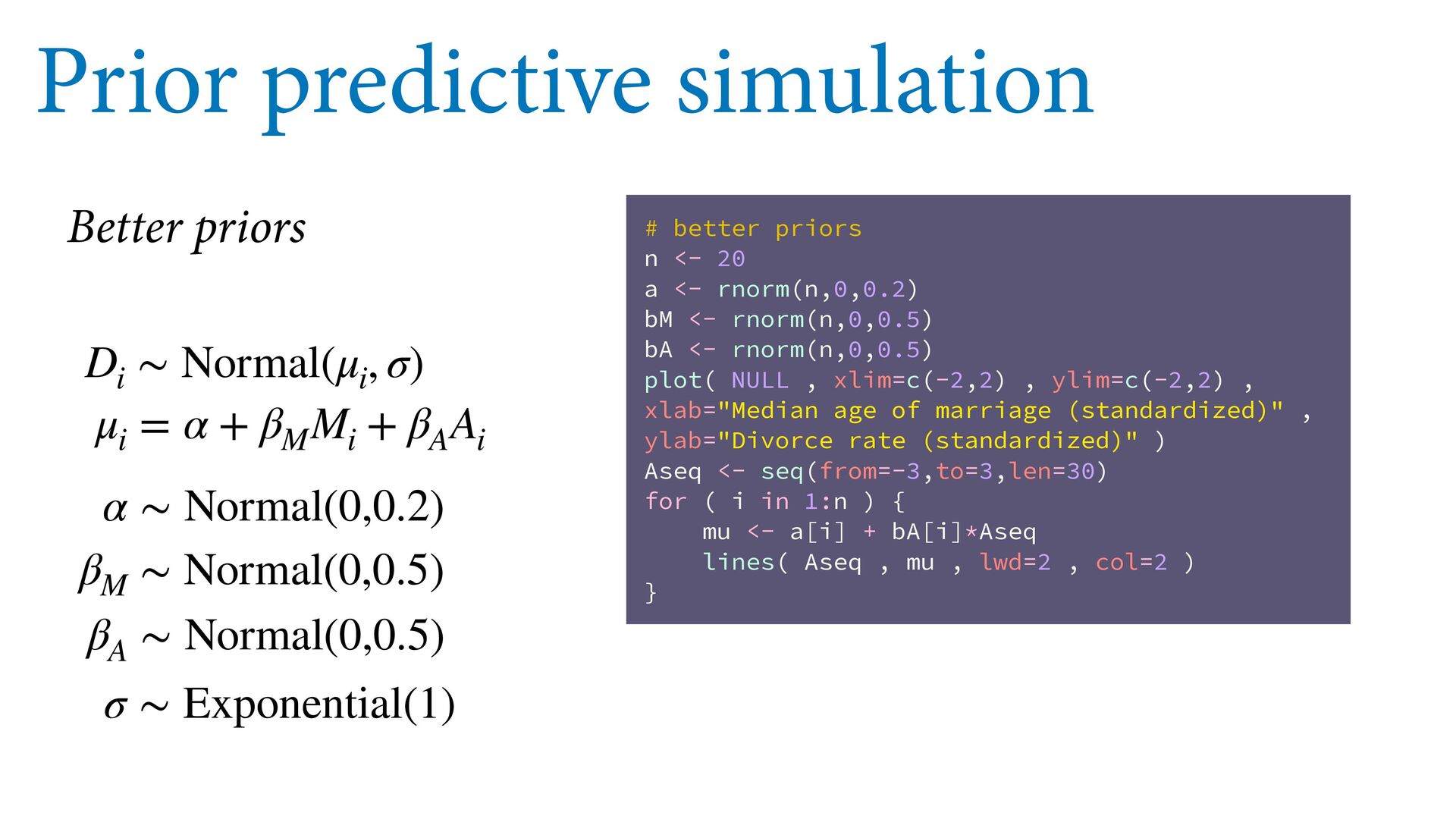
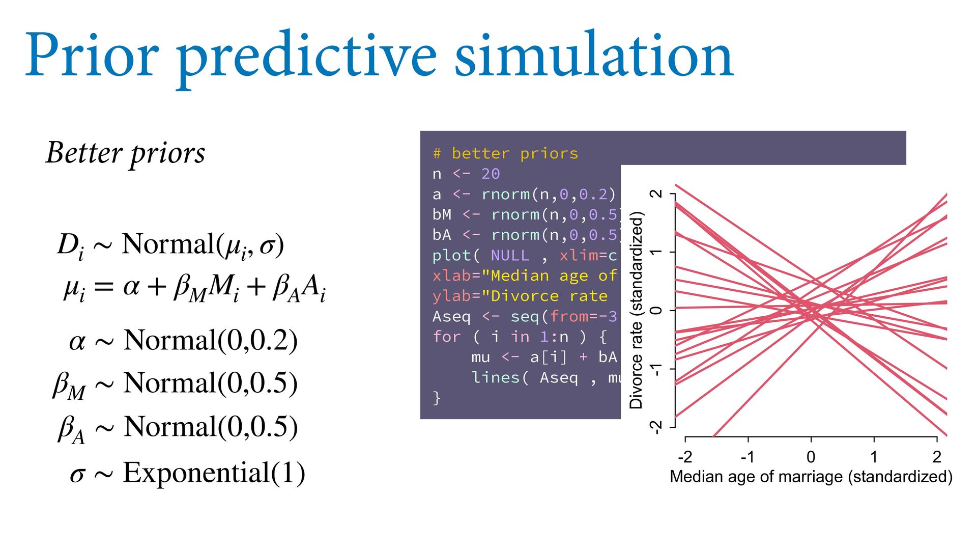
<- rnorm(n,0,0.5) bA <- rnorm(n,0,0.5) plot( NULL , xlim=c(-2,2) , ylim=c(-2,2) , xlab="Median age of marriage (standardized)" , ylab="Divorce rate (standardized)" ) Aseq <- seq(from=-3,to=3,len=30) for ( i in 1:n ) { mu <- a[i] + bA[i]*Aseq lines( Aseq , mu , lwd=2 , col=2 ) } Prior predictive simulation μ i = α + β M M i + β A A i D i ∼ Normal(μ i , σ) α ∼ Normal(0,0.2) β M ∼ Normal(0,0.5) β A ∼ Normal(0,0.5) σ ∼ Exponential(1) Better priors
<- rnorm(n,0,0.5) bA <- rnorm(n,0,0.5) plot( NULL , xlim=c(-2,2) , ylim=c(-2,2) , xlab="Median age of marriage (standardized)" , ylab="Divorce rate (standardized)" ) Aseq <- seq(from=-3,to=3,len=30) for ( i in 1:n ) { mu <- a[i] + bA[i]*Aseq lines( Aseq , mu , lwd=2 , col=2 ) } Prior predictive simulation μ i = α + β M M i + β A A i D i ∼ Normal(μ i , σ) α ∼ Normal(0,0.2) β M ∼ Normal(0,0.5) β A ∼ Normal(0,0.5) σ ∼ Exponential(1) Better priors -2 -1 0 1 2 -2 -1 0 1 2 Median age of marriage (standardized) Divorce rate (standardized)
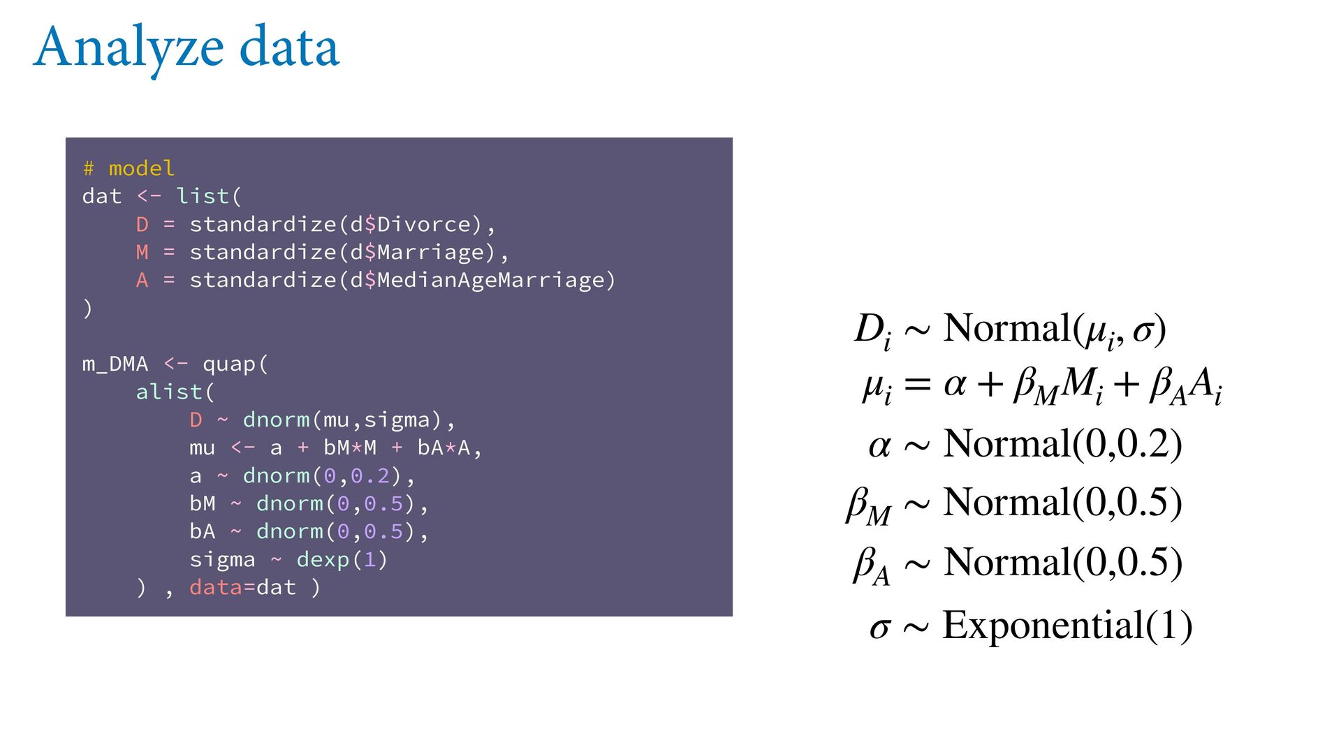
standardize(d$Marriage), A = standardize(d$MedianAgeMarriage) ) m_DMA <- quap( alist( D ~ dnorm(mu,sigma), mu <- a + bM*M + bA*A, a ~ dnorm(0,0.2), bM ~ dnorm(0,0.5), bA ~ dnorm(0,0.5), sigma ~ dexp(1) ) , data=dat ) μ i = α + β M M i + β A A i D i ∼ Normal(μ i , σ) α ∼ Normal(0,0.2) β M ∼ Normal(0,0.5) β A ∼ Normal(0,0.5) σ ∼ Exponential(1) Analyze data
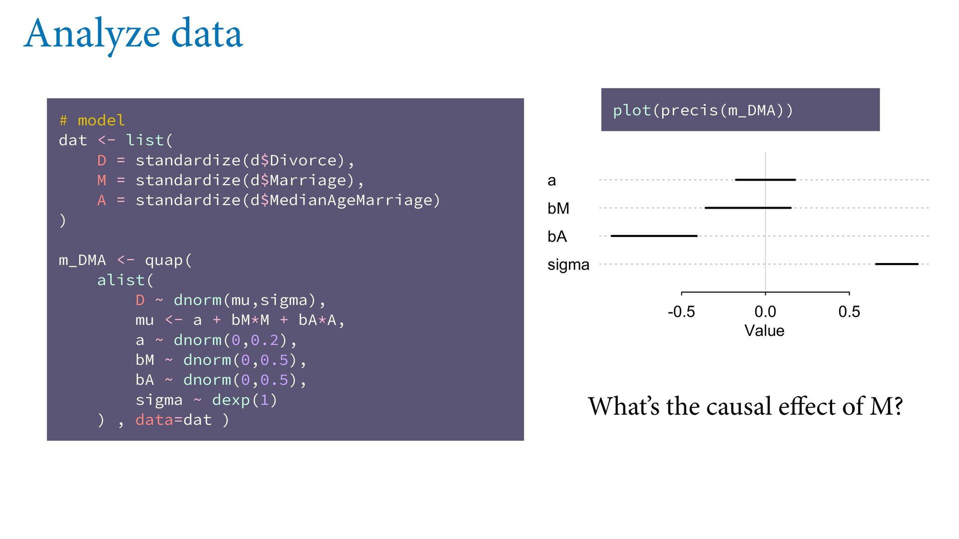
standardize(d$Marriage), A = standardize(d$MedianAgeMarriage) ) m_DMA <- quap( alist( D ~ dnorm(mu,sigma), mu <- a + bM*M + bA*A, a ~ dnorm(0,0.2), bM ~ dnorm(0,0.5), bA ~ dnorm(0,0.5), sigma ~ dexp(1) ) , data=dat ) sigma bA bM a -0.5 0.0 0.5 Value plot(precis(m_DMA)) What’s the causal effect of M? Analyze data
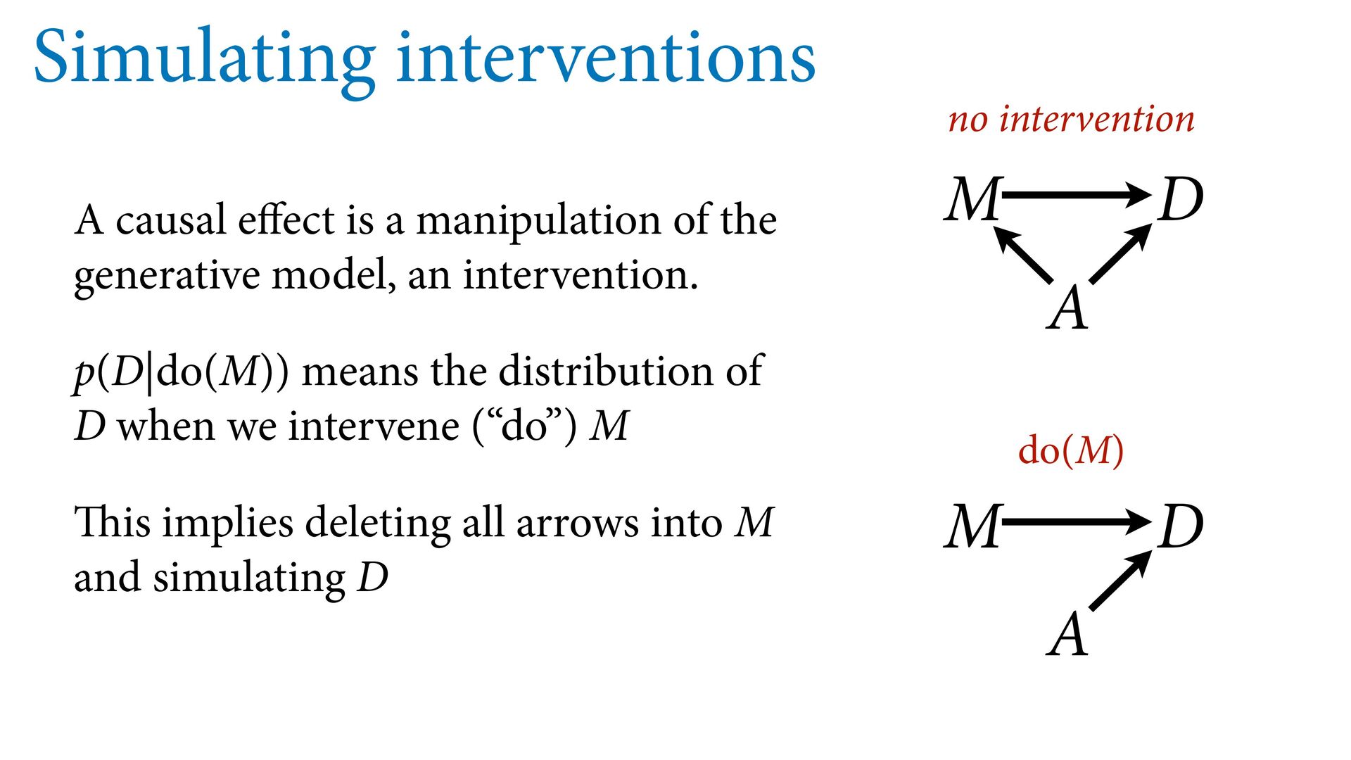
generative model, an intervention. p(D|do(M)) means the distribution of D when we intervene (“do”) M This implies deleting all arrows into M and simulating D M D A M D A no intervention do(M)
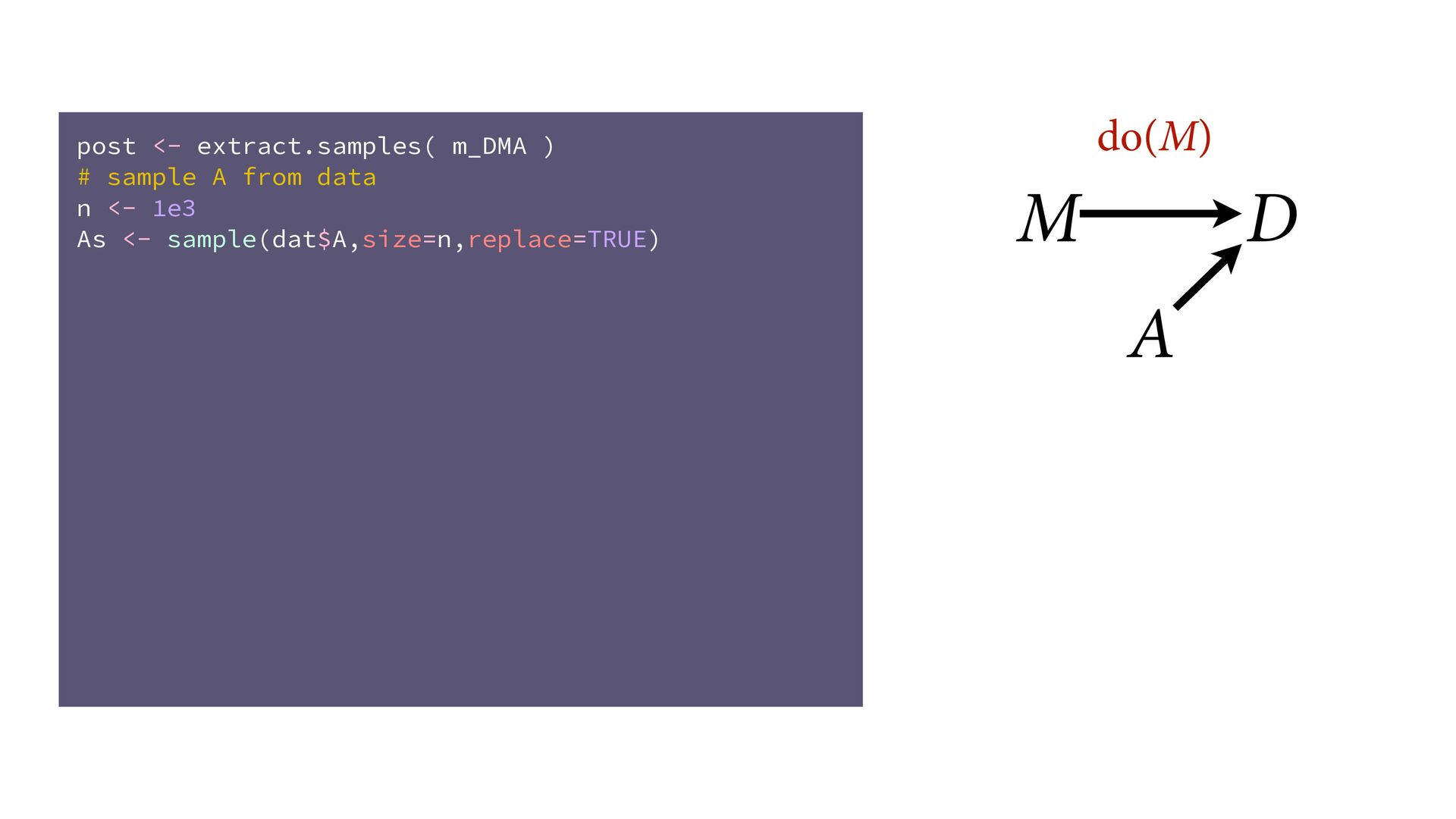
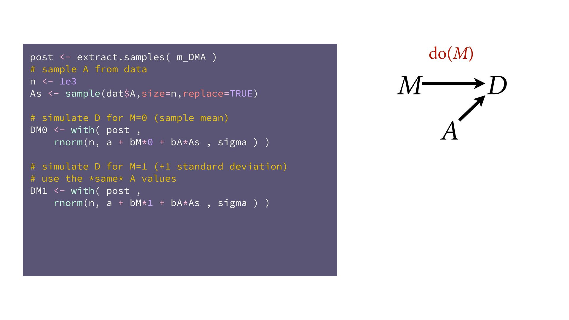
sample A from data n <- 1e3 As <- sample(dat$A,size=n,replace=TRUE) # simulate D for M=0 (sample mean) DM0 <- with( post , rnorm(n, a + bM*0 + bA*As , sigma ) ) # simulate D for M=1 (+1 standard deviation) # use the *same* A values DM1 <- with( post , rnorm(n, a + bM*1 + bA*As , sigma ) ) # contrast M10_contrast <- DM1 - DM0 dens(M10_contrast,lwd=4,col=2,xlab="effect of 1sd increase in M" )
sample A from data n <- 1e3 As <- sample(dat$A,size=n,replace=TRUE) # simulate D for M=0 (sample mean) DM0 <- with( post , rnorm(n, a + bM*0 + bA*As , sigma ) ) # simulate D for M=1 (+1 standard deviation) # use the *same* A values DM1 <- with( post , rnorm(n, a + bM*1 + bA*As , sigma ) ) # contrast M10_contrast <- DM1 - DM0 dens(M10_contrast,lwd=4,col=2,xlab="effect of 1sd increase in M" )
sample A from data n <- 1e3 As <- sample(dat$A,size=n,replace=TRUE) # simulate D for M=0 (sample mean) DM0 <- with( post , rnorm(n, a + bM*0 + bA*As , sigma ) ) # simulate D for M=1 (+1 standard deviation) # use the *same* A values DM1 <- with( post , rnorm(n, a + bM*1 + bA*As , sigma ) ) # contrast M10_contrast <- DM1 - DM0 dens(M10_contrast,lwd=4,col=2,xlab="effect of 1sd increase in M" )
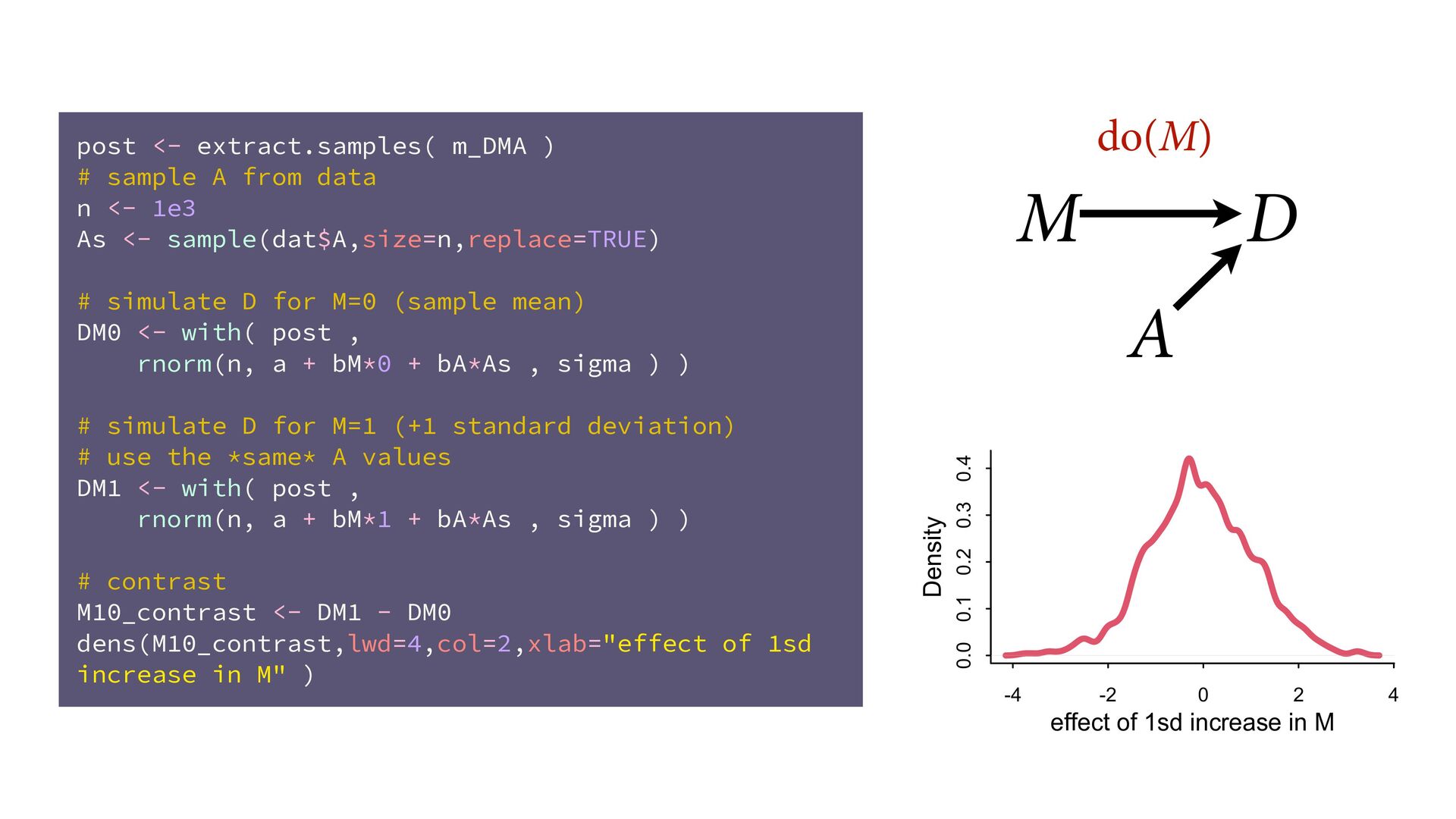
sample A from data n <- 1e3 As <- sample(dat$A,size=n,replace=TRUE) # simulate D for M=0 (sample mean) DM0 <- with( post , rnorm(n, a + bM*0 + bA*As , sigma ) ) # simulate D for M=1 (+1 standard deviation) # use the *same* A values DM1 <- with( post , rnorm(n, a + bM*1 + bA*As , sigma ) ) # contrast M10_contrast <- DM1 - DM0 dens(M10_contrast,lwd=4,col=2,xlab="effect of 1sd increase in M" ) -4 -2 0 2 4 0.0 0.1 0.2 0.3 0.4 effect of 1sd increase in M Density
estimate causal effect of A, p(D|do(A))? No arrows to delete for intervention Fit new model that ignores M, then simulate any intervention you like Why does ignoring M work? Because A –> M –> D is a “pipe”
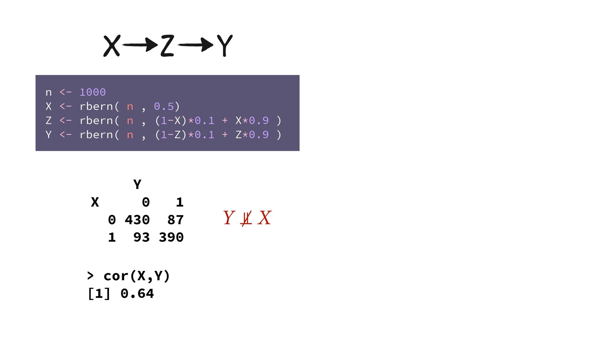
Z = 0 Y X 0 1 0 422 39 1 53 5 Z = 1 Y X 0 1 0 8 48 1 40 385 X Z Y n <- 1000 X <- rbern( n , 0.5) Z <- rbern( n , (1-X)*0.1 + X*0.9 ) Y <- rbern( n , (1-Z)*0.1 + Z*0.9 ) > cor(X,Y) [1] 0.64 > cor(X[Z==0],Y[Z==0]) [1] 0.002 > cor(X[Z==1],Y[Z==1]) [1] 0.052 Y ⫫ X Y ⫫ X | Z
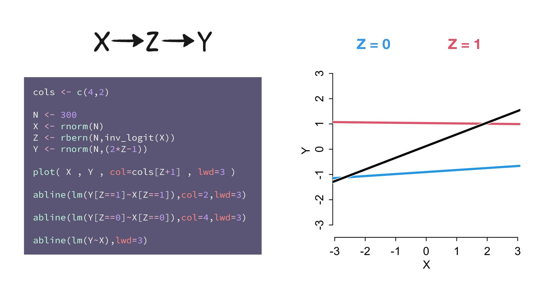
<- 300 X <- rnorm(N) Z <- rbern(N,inv_logit(X)) Y <- rnorm(N,(2*Z-1)) plot( X , Y , col=cols[Z+1] , lwd=3 ) abline(lm(Y[Z==1]~X[Z==1]),col=2,lwd=3) abline(lm(Y[Z==0]~X[Z==0]),col=4,lwd=3) abline(lm(Y~X),lwd=3) X Z Y -3 -2 -1 0 1 2 3 -3 -2 -1 0 1 2 3 X Y
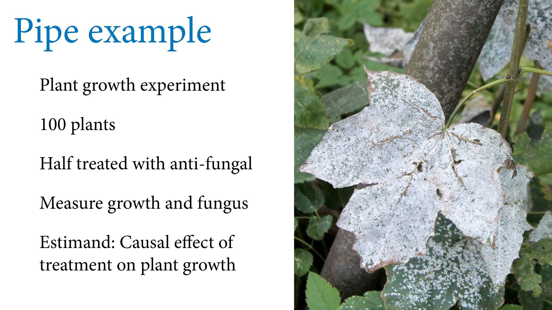
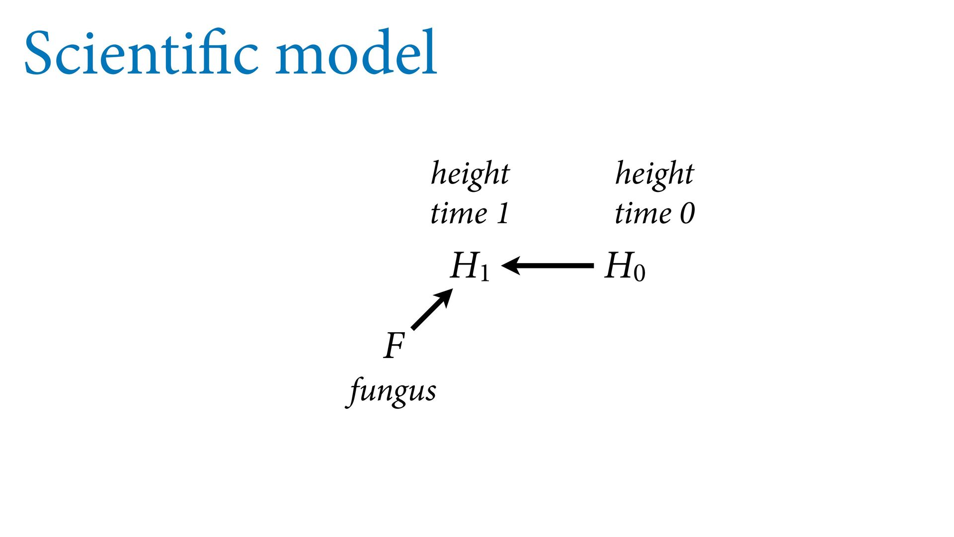
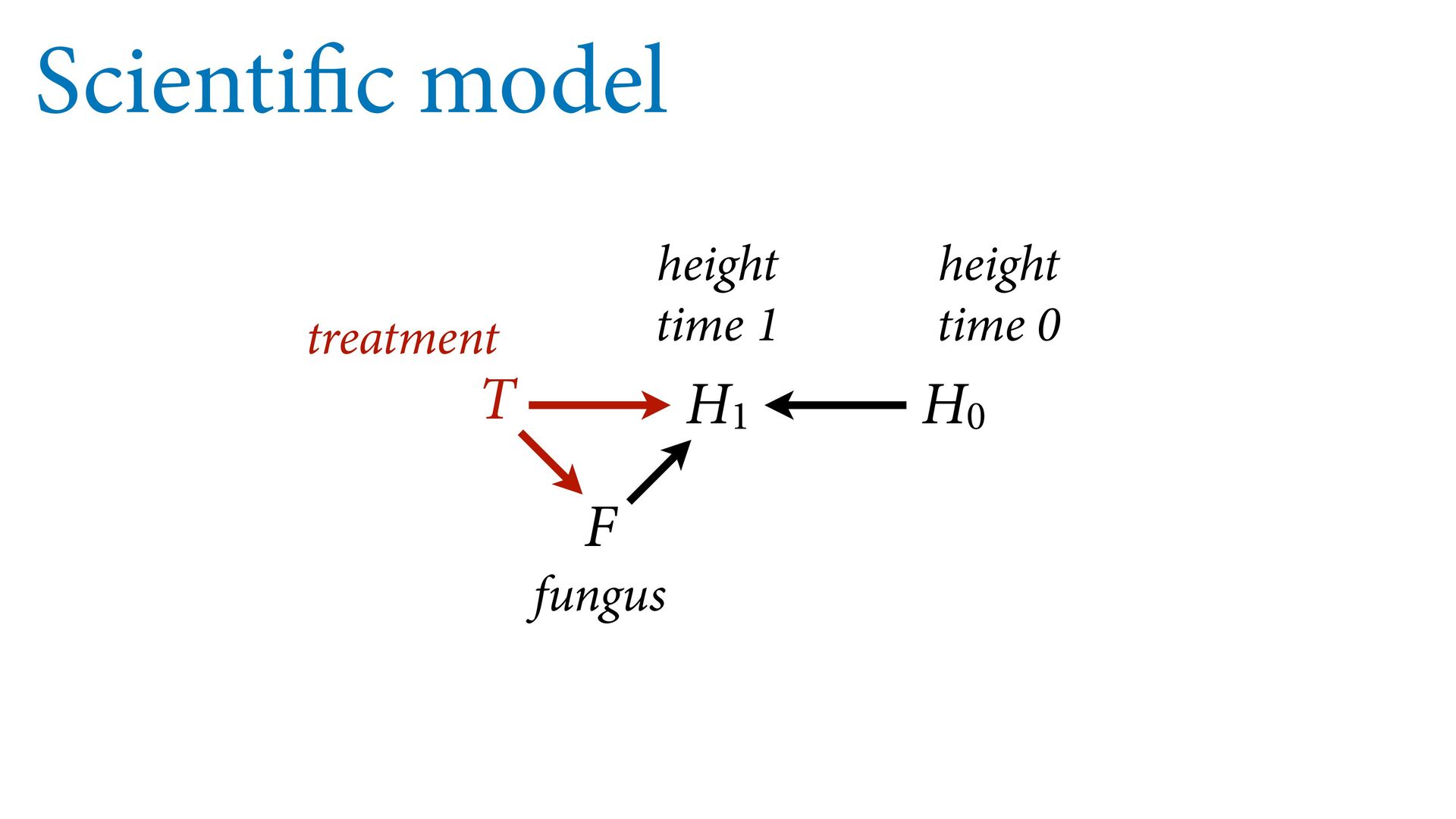
T –> F –> H1 is a pipe Should we stratify by F? NO — that would block the pipe See pages 170–175 for complete example H0 H1 T F The treatment must flow
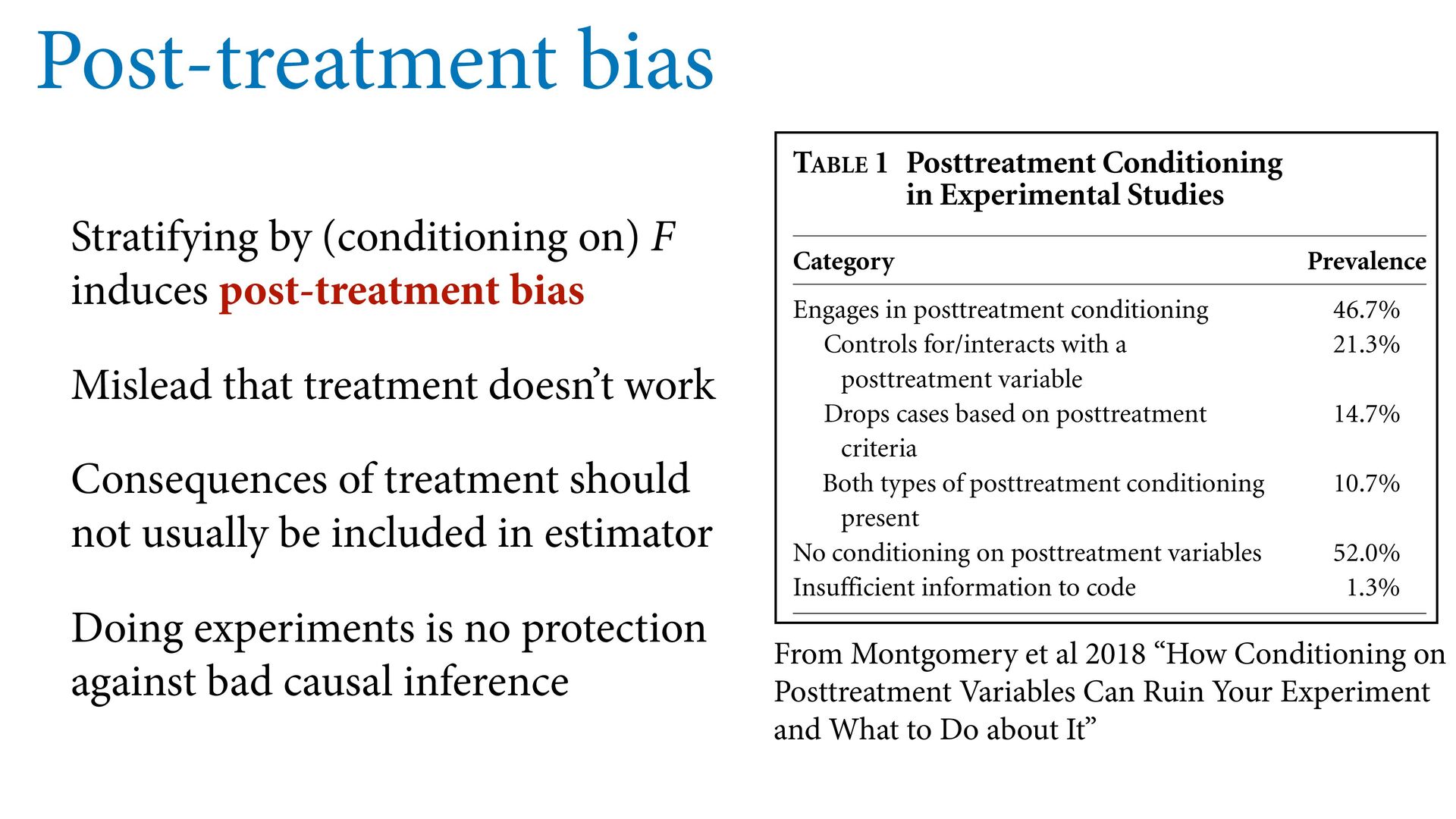
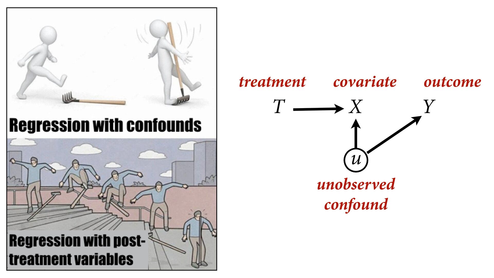
Mislead that treatment doesn’t work Consequences of treatment should not usually be included in estimator Doing experiments is no protection against bad causal inference STOP CONDITIONING ON POSTTREATMENT VARIABLES IN EXPERIMENTS 761 unlikely to hold in real-world settings. In short, condi- tioning on posttreatment variables can ruin experiments; we should not do it. Though the dangers of posttreatment bias have long been recognized in the fields of statistics, econometrics, and political methodology (e.g., Acharya, Blackwell, and Sen 2016; Elwert and Winship 2014; King and Zeng 2006; Rosenbaum 1984; Wooldridge 2005), there is still signif- icant confusion in the wider discipline about its sources and consequences. In this article, we therefore seek to provide the most comprehensive and accessible account to date of the sources, magnitude, and frequency of post- treatment bias in experimental political science research. We first identify common practices that lead to posttreat- mentconditioninganddocumenttheirprevalenceinarti- cles published in the field’s top journals. We then provide analyticalresultsthatexplainhowposttreatmentbiascon- taminates experimental analyses and demonstrate how it can distort treatment effect estimates using data from TABLE 1 Posttreatment Conditioning in Experimental Studies Category Prevalence Engages in posttreatment conditioning 46.7% Controls for/interacts with a posttreatment variable 21.3% Drops cases based on posttreatment criteria 14.7% Both types of posttreatment conditioning present 10.7% No conditioning on posttreatment variables 52.0% Insufficient information to code 1.3% Note: The sample consists of 2012–14 articles in the American Po- litical Science Review, the American Journal of Political Science, and the Journal of Politics including a survey, field, laboratory, or lab- in-the-field experiment (n = 75). avoid posttreatment bias. In many cases, the usefulness From Montgomery et al 2018 “How Conditioning on Posttreatment Variables Can Ruin Your Experiment and What to Do about It”
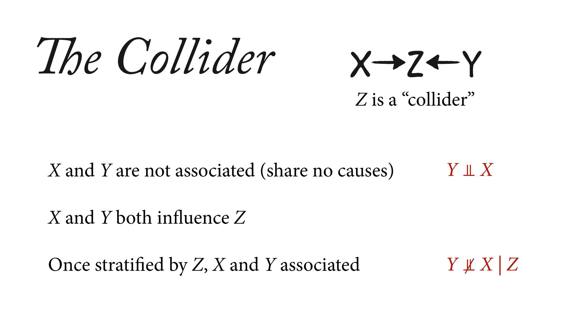
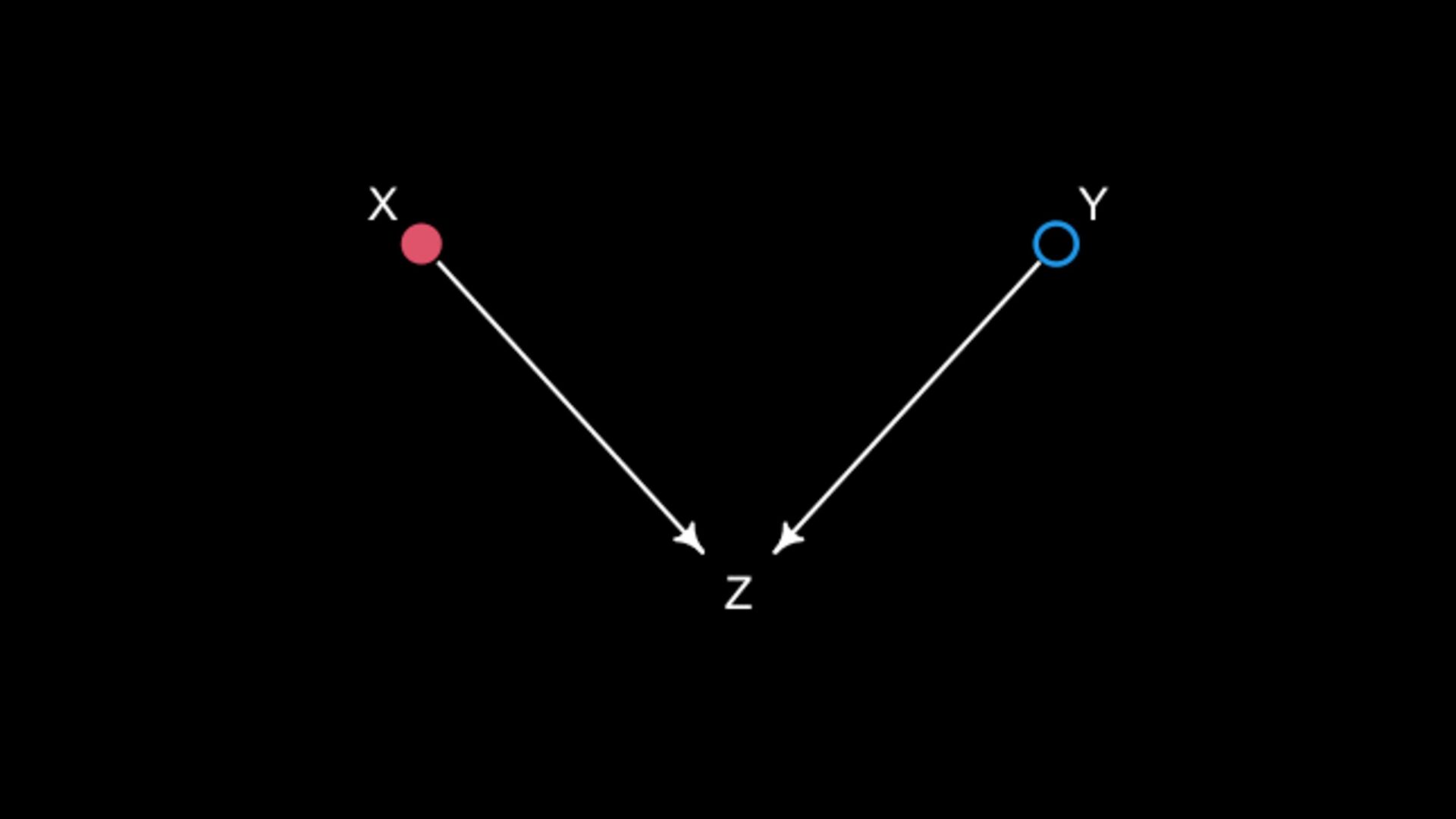
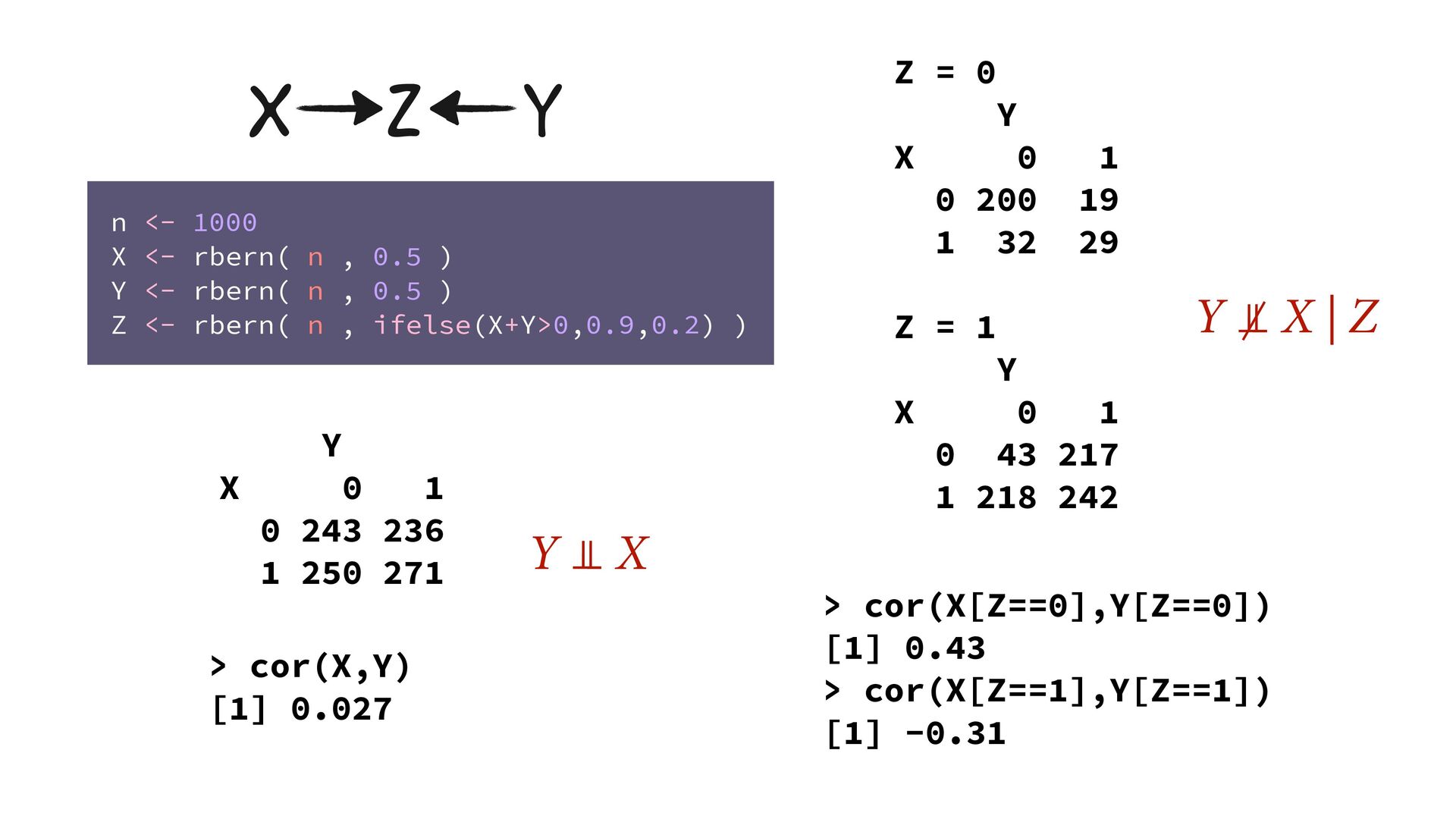
243 236 1 250 271 Z = 0 Y X 0 1 0 200 19 1 32 29 Z = 1 Y X 0 1 0 43 217 1 218 242 X Z Y n <- 1000 X <- rbern( n , 0.5 ) Y <- rbern( n , 0.5 ) Z <- rbern( n , ifelse(X+Y>0,0.9,0.2) ) > cor(X,Y) [1] 0.027 > cor(X[Z==0],Y[Z==0]) [1] 0.43 > cor(X[Z==1],Y[Z==1]) [1] -0.31 Y ⫫ X
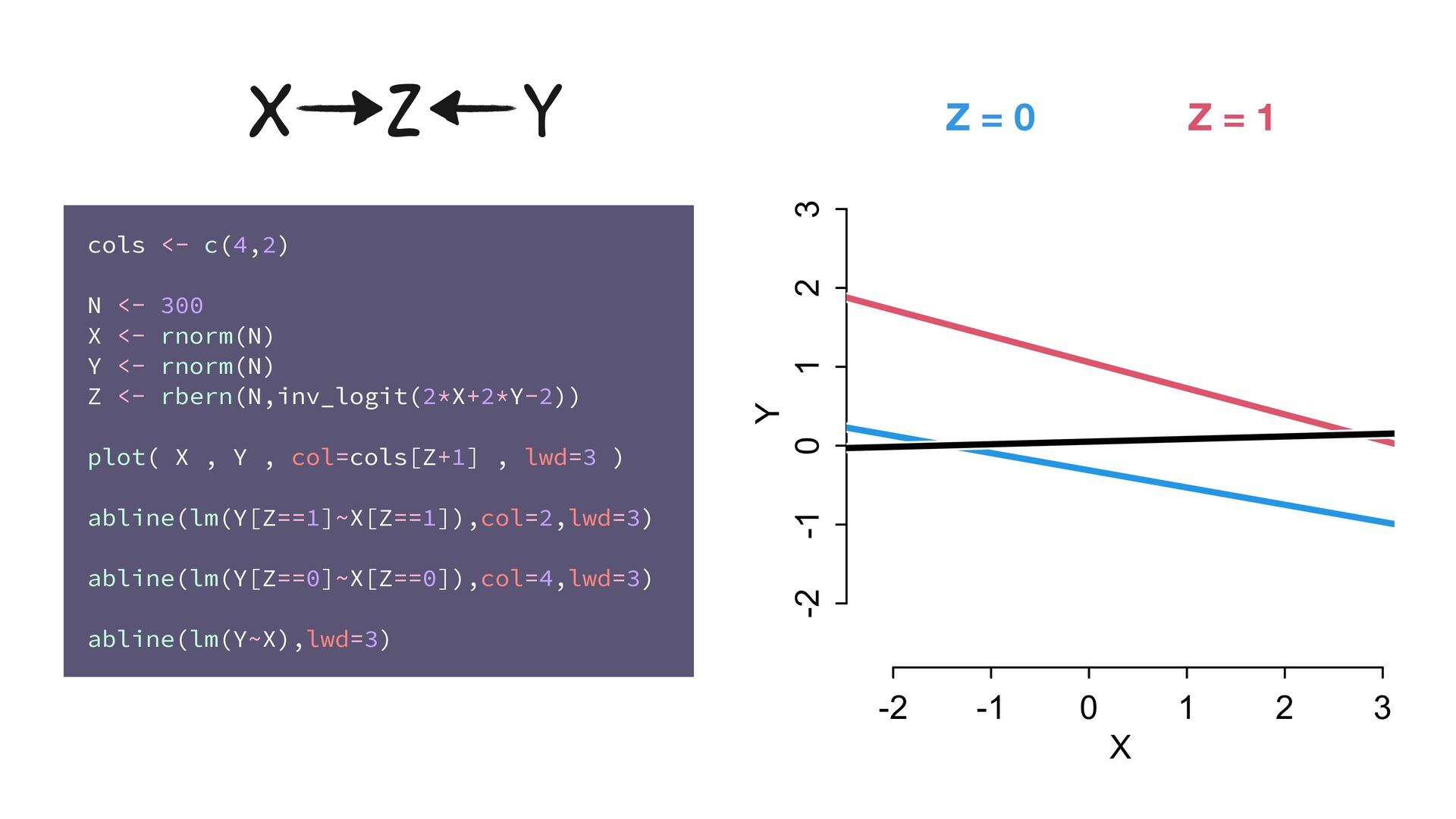
<- 300 X <- rnorm(N) Y <- rnorm(N) Z <- rbern(N,inv_logit(2*X+2*Y-2)) plot( X , Y , col=cols[Z+1] , lwd=3 ) abline(lm(Y[Z==1]~X[Z==1]),col=2,lwd=3) abline(lm(Y[Z==0]~X[Z==0]),col=4,lwd=3) abline(lm(Y~X),lwd=3) X Z Y -2 -1 0 1 2 3 -2 -1 0 1 2 3 X Y
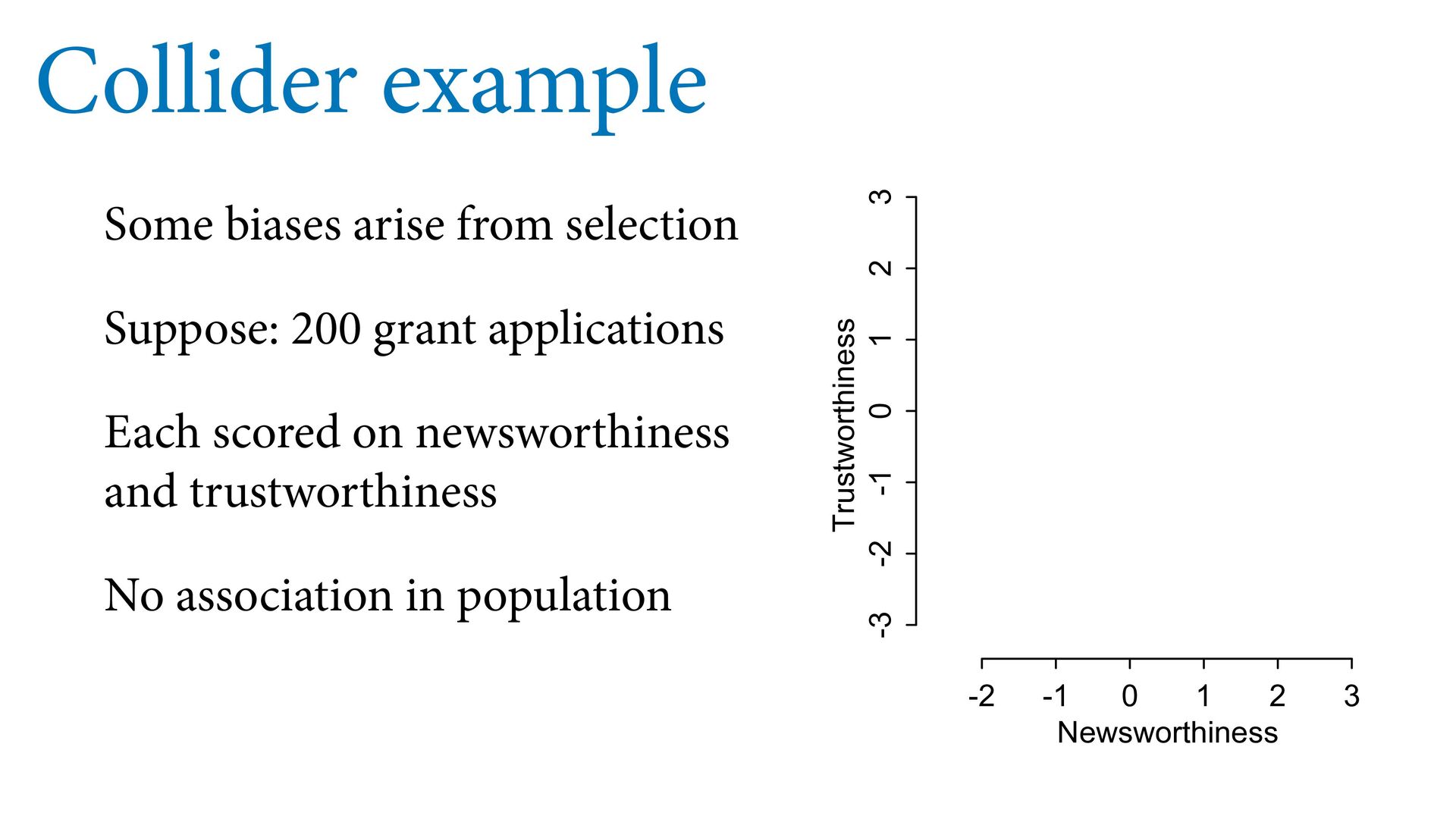
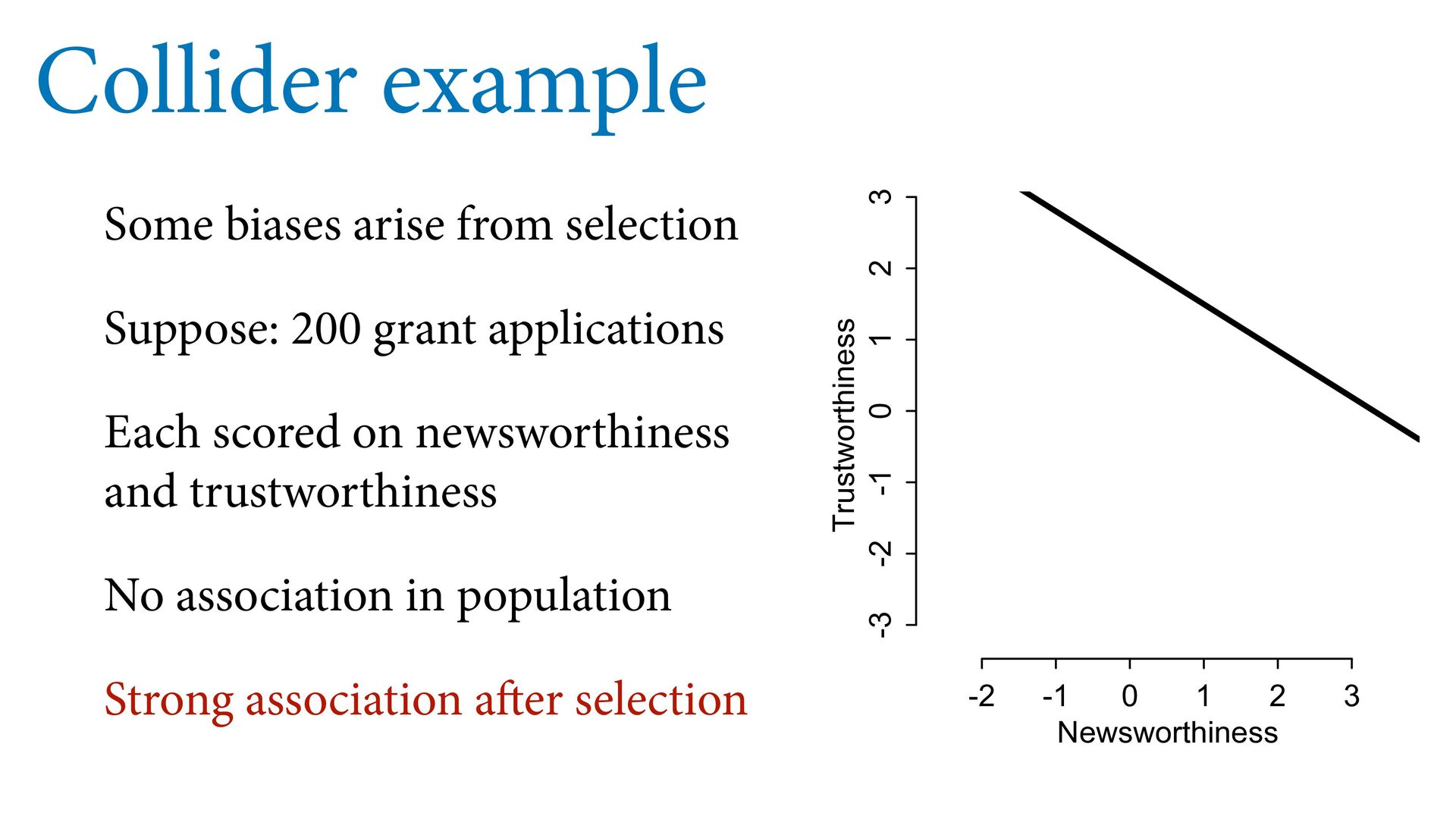
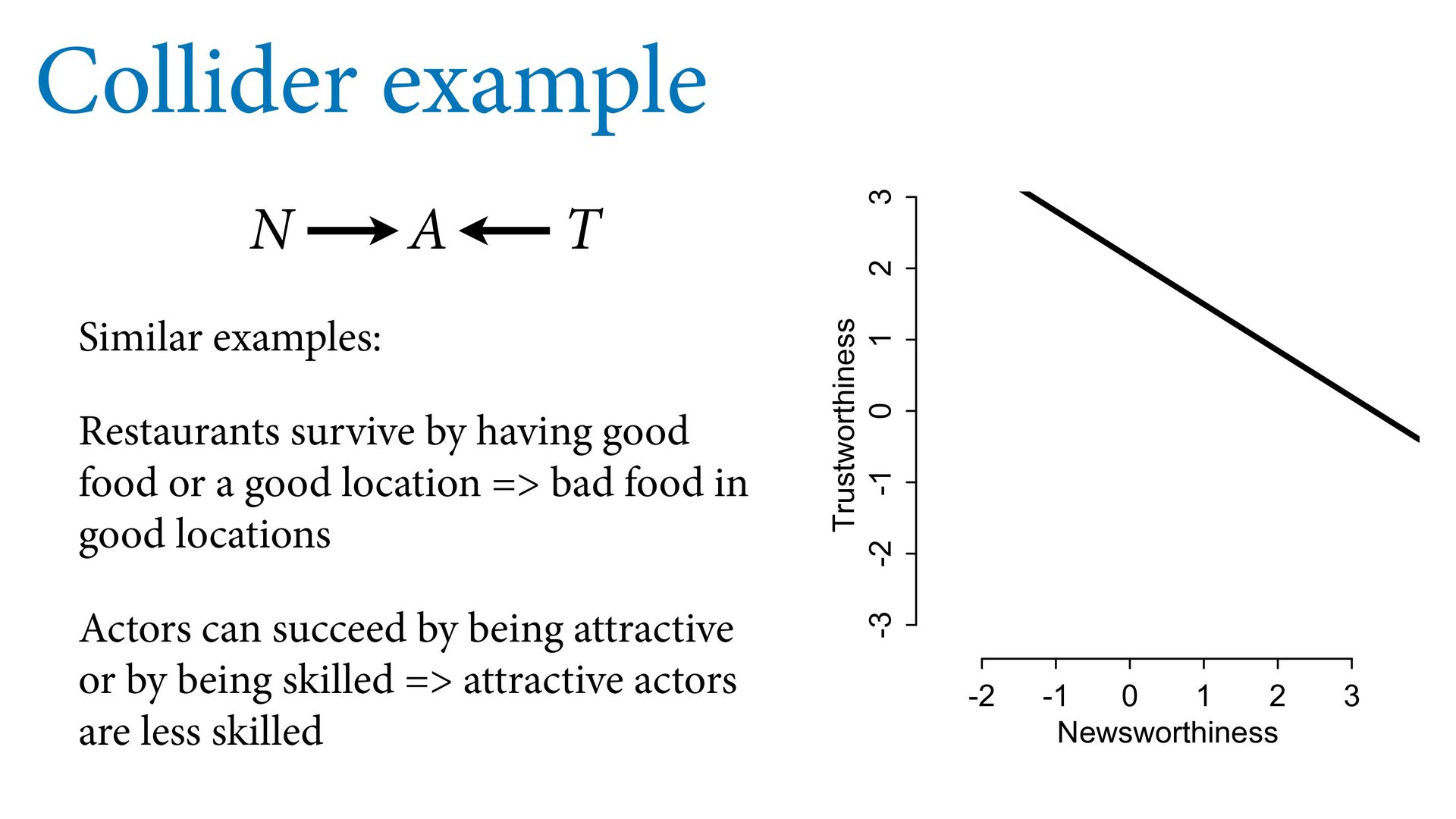
1 2 3 Newsworthiness Trustworthiness Collider example Some biases arise from selection Suppose: 200 grant applications Each scored on newsworthiness and trustworthiness No association in population Strong association after selection
1 2 3 Newsworthiness Trustworthiness Collider example Some biases arise from selection Suppose: 200 grant applications Each scored on newsworthiness and trustworthiness No association in population Strong association after selection
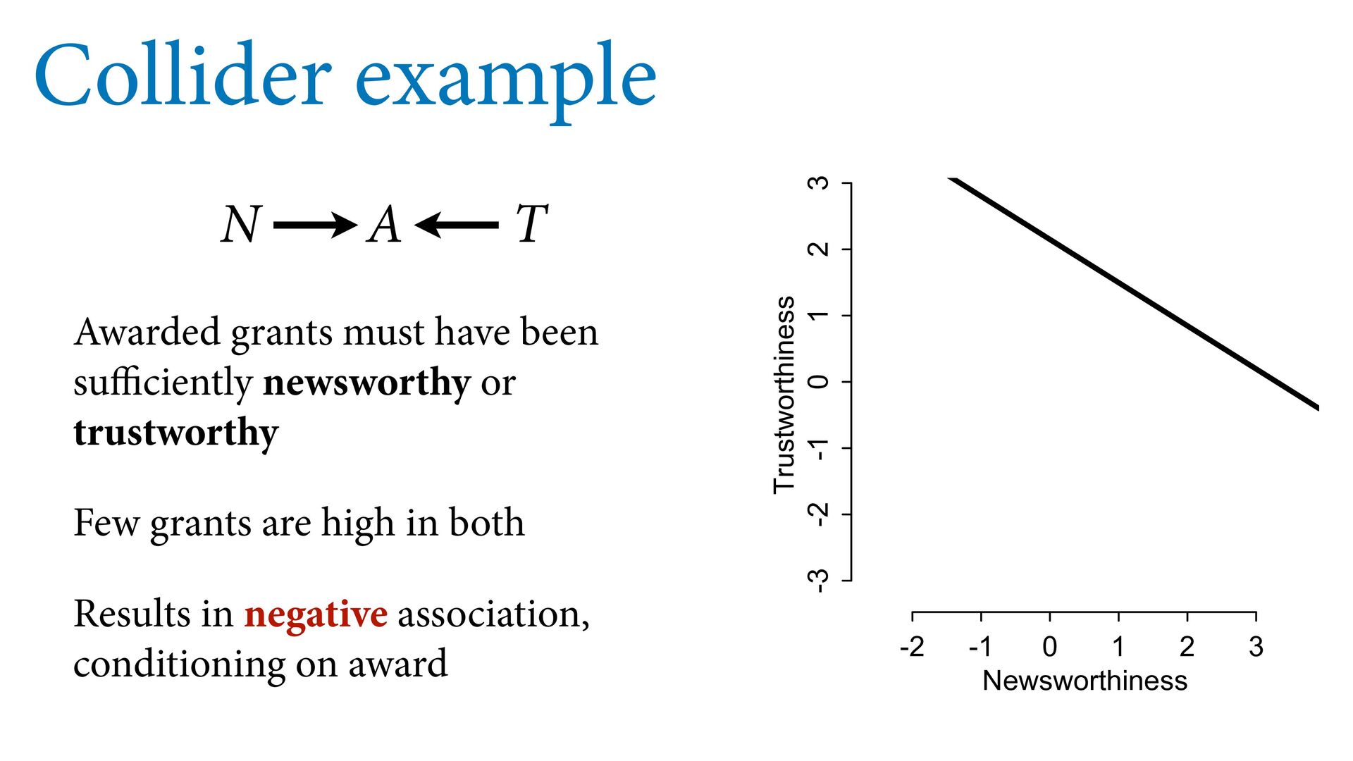
trustworthy Few grants are high in both Results in negative association, conditioning on award N T A -2 -1 0 1 2 3 -3 -2 -1 0 1 2 3 Newsworthiness Trustworthiness
or a good location => bad food in good locations Actors can succeed by being attractive or by being skilled => attractive actors are less skilled N T A -2 -1 0 1 2 3 -3 -2 -1 0 1 2 3 Newsworthiness Trustworthiness
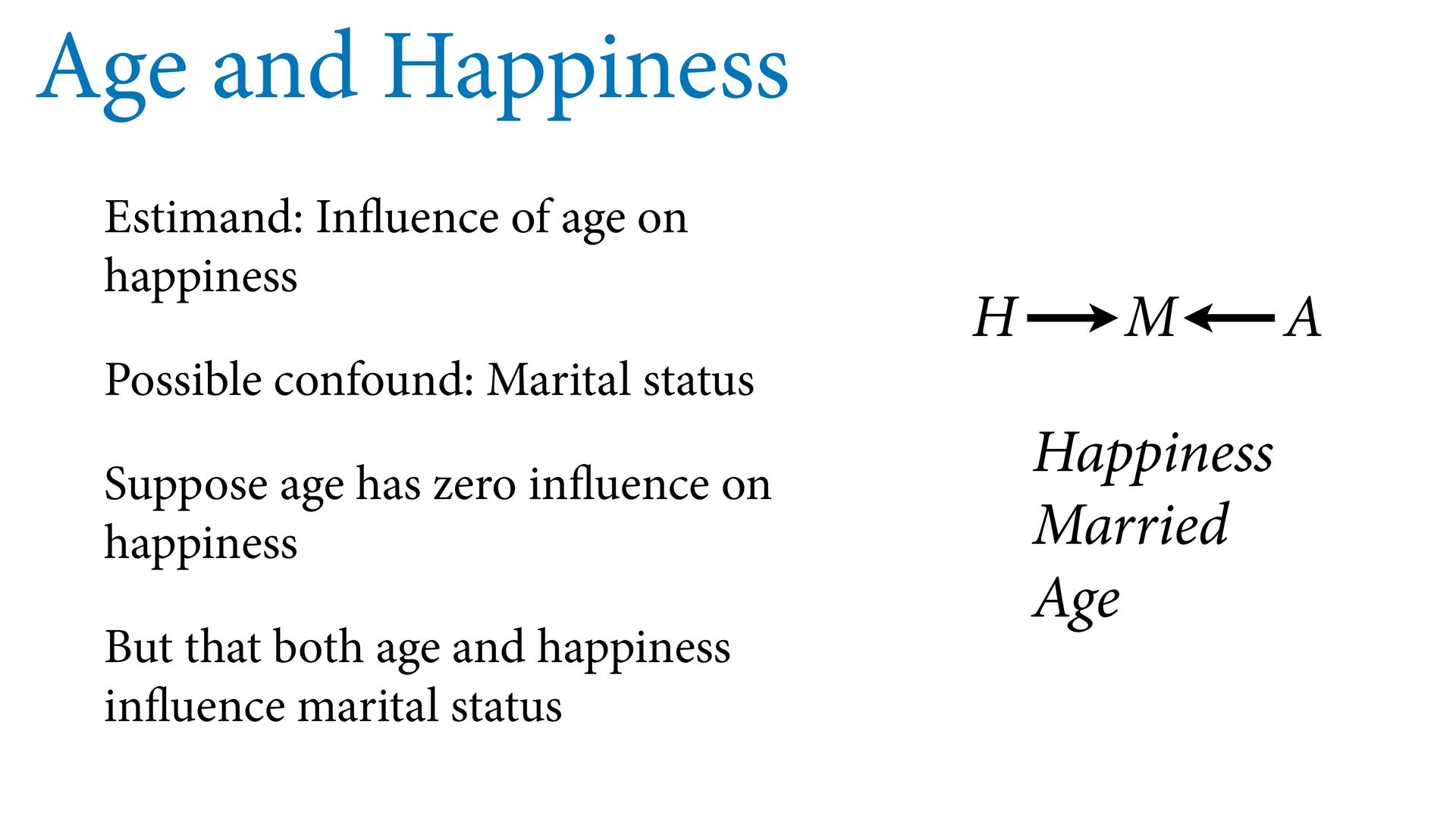
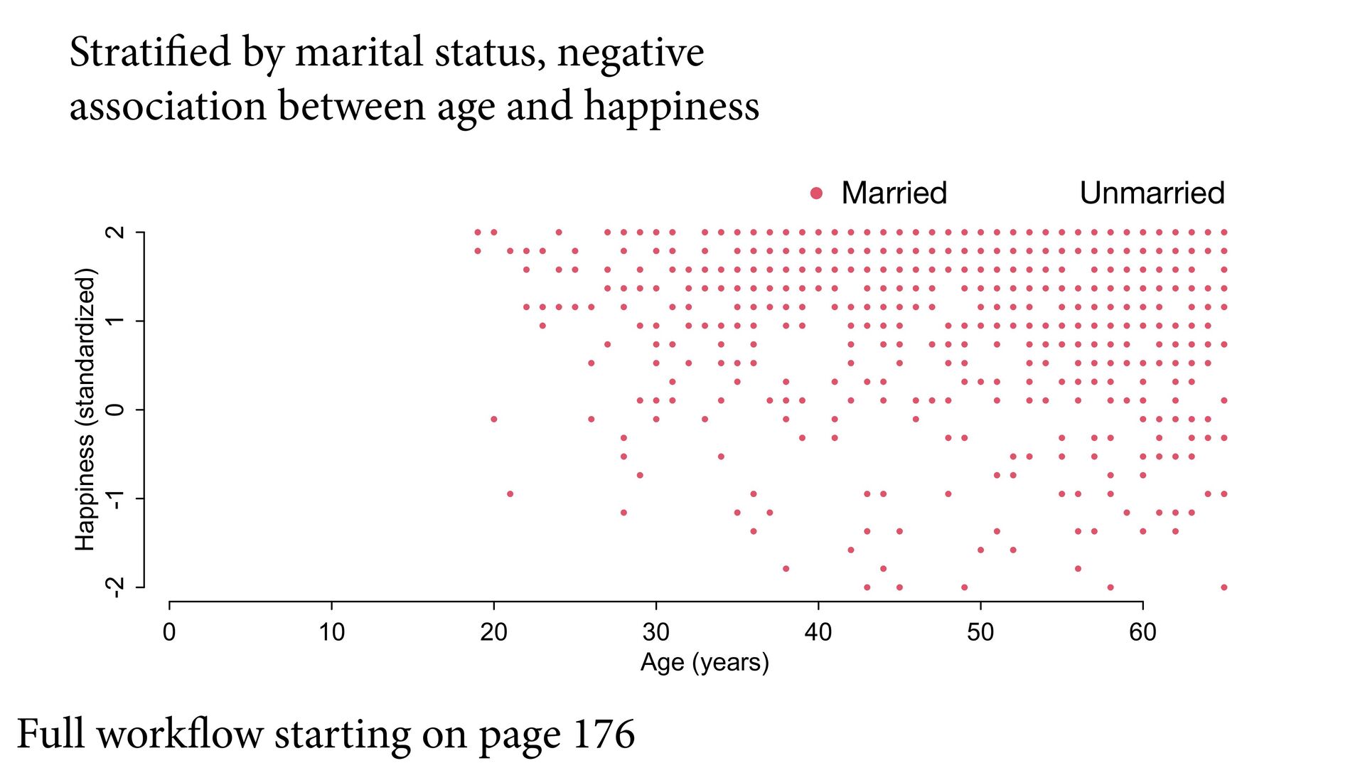
confound: Marital status Suppose age has zero influence on happiness But that both age and happiness influence marital status H A M Happiness Married Age
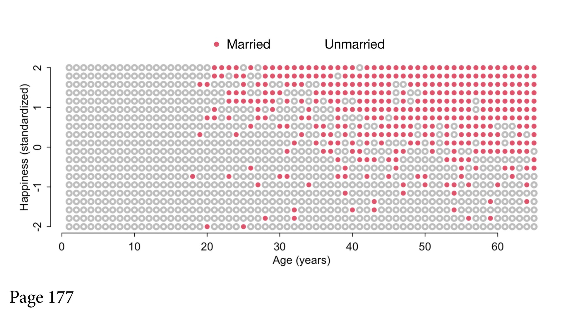
1 2 Age (years) Happiness (standardized) Full workflow starting on page 176 Stratified by marital status, negative association between age and happiness Married Unmarried
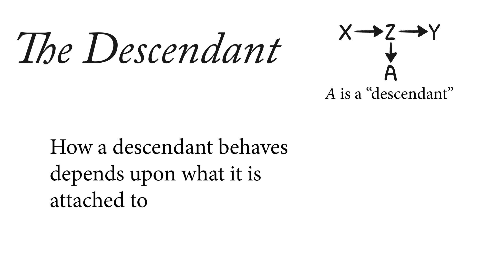
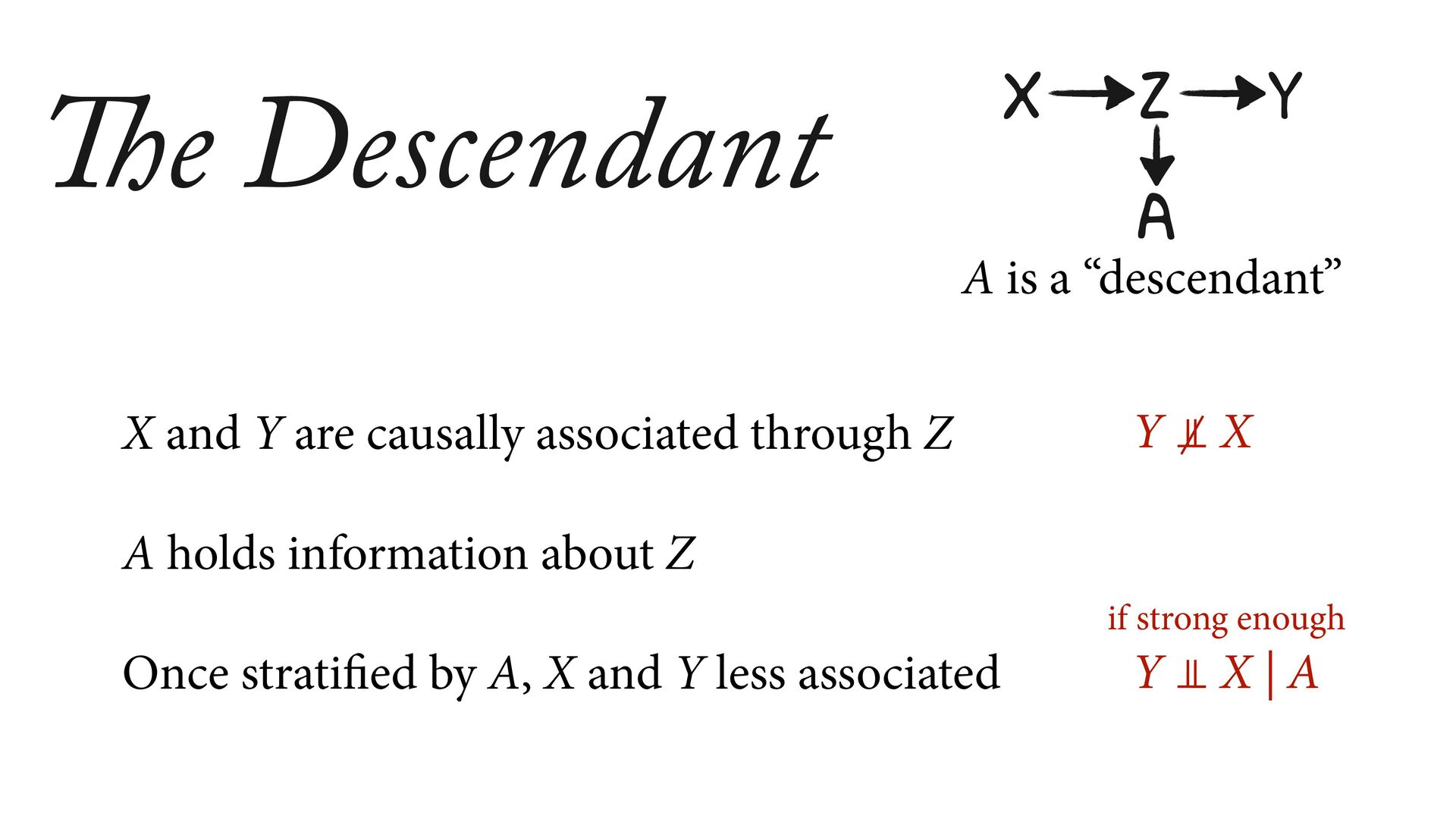
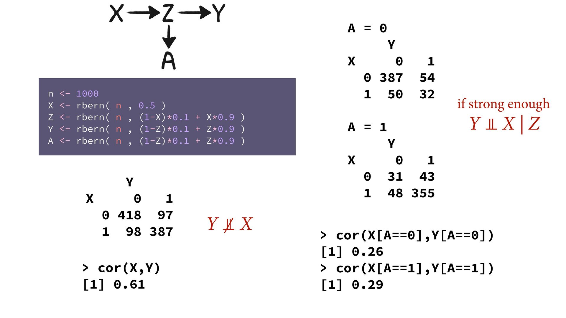
are causally associated through Z A holds information about Z Once stratified by A, X and Y less associated Y ⫫ X A is a “descendant” X Z Y A if strong enough
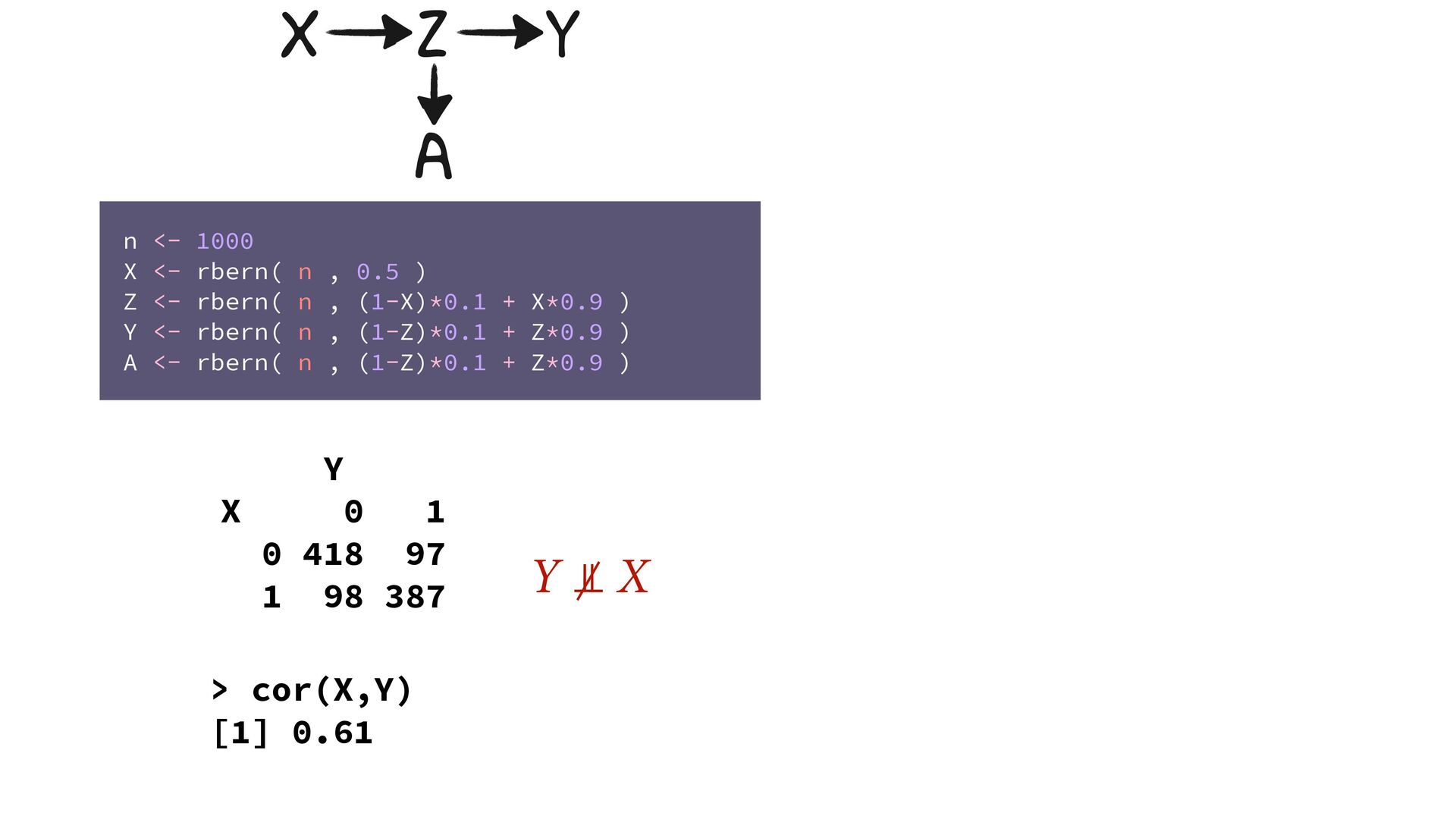
> cor(X,Y) [1] 0.61 Y ⫫ X n <- 1000 X <- rbern( n , 0.5 ) Z <- rbern( n , (1-X)*0.1 + X*0.9 ) Y <- rbern( n , (1-Z)*0.1 + Z*0.9 ) A <- rbern( n , (1-Z)*0.1 + Z*0.9 ) X Z Y A
418 97 1 98 387 A = 0 Y X 0 1 0 387 54 1 50 32 A = 1 Y X 0 1 0 31 43 1 48 355 > cor(X,Y) [1] 0.61 > cor(X[A==0],Y[A==0]) [1] 0.26 > cor(X[A==1],Y[A==1]) [1] 0.29 Y ⫫ X n <- 1000 X <- rbern( n , 0.5 ) Z <- rbern( n , (1-X)*0.1 + X*0.9 ) Y <- rbern( n , (1-Z)*0.1 + Z*0.9 ) A <- rbern( n , (1-Z)*0.1 + Z*0.9 ) X Z Y A if strong enough