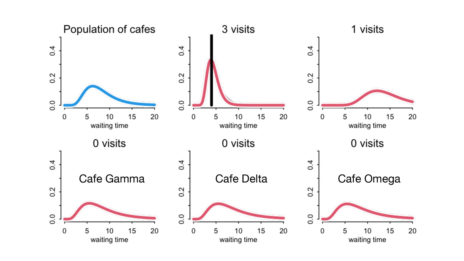
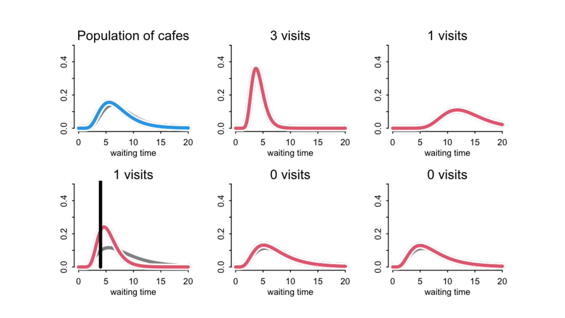
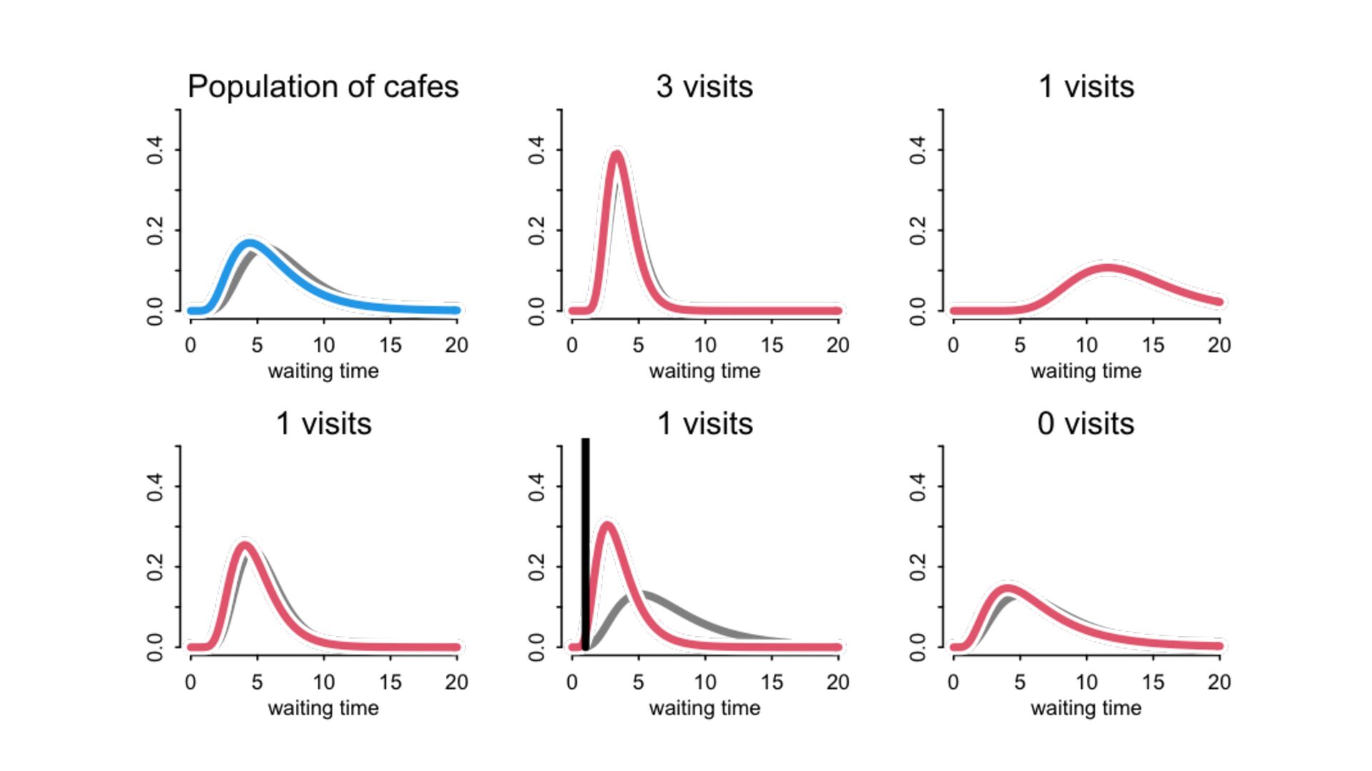
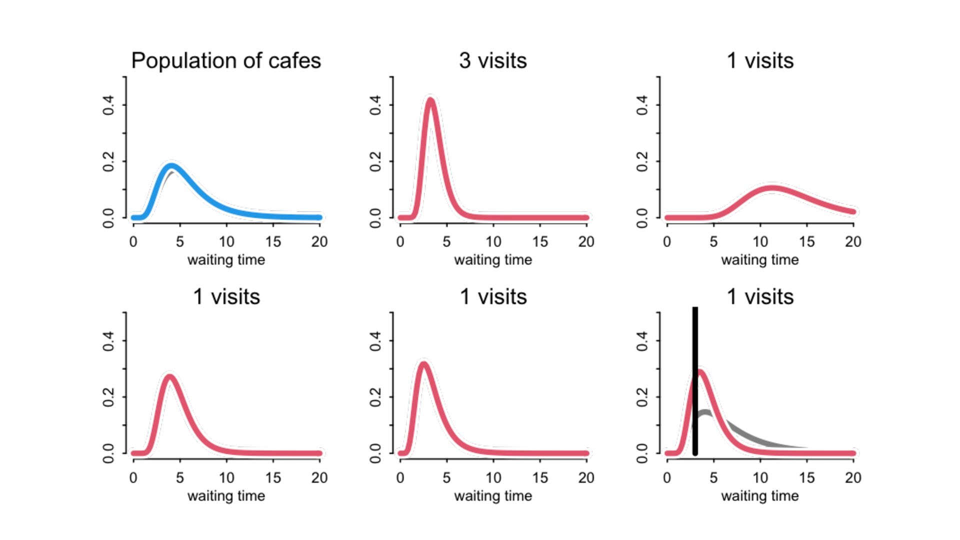
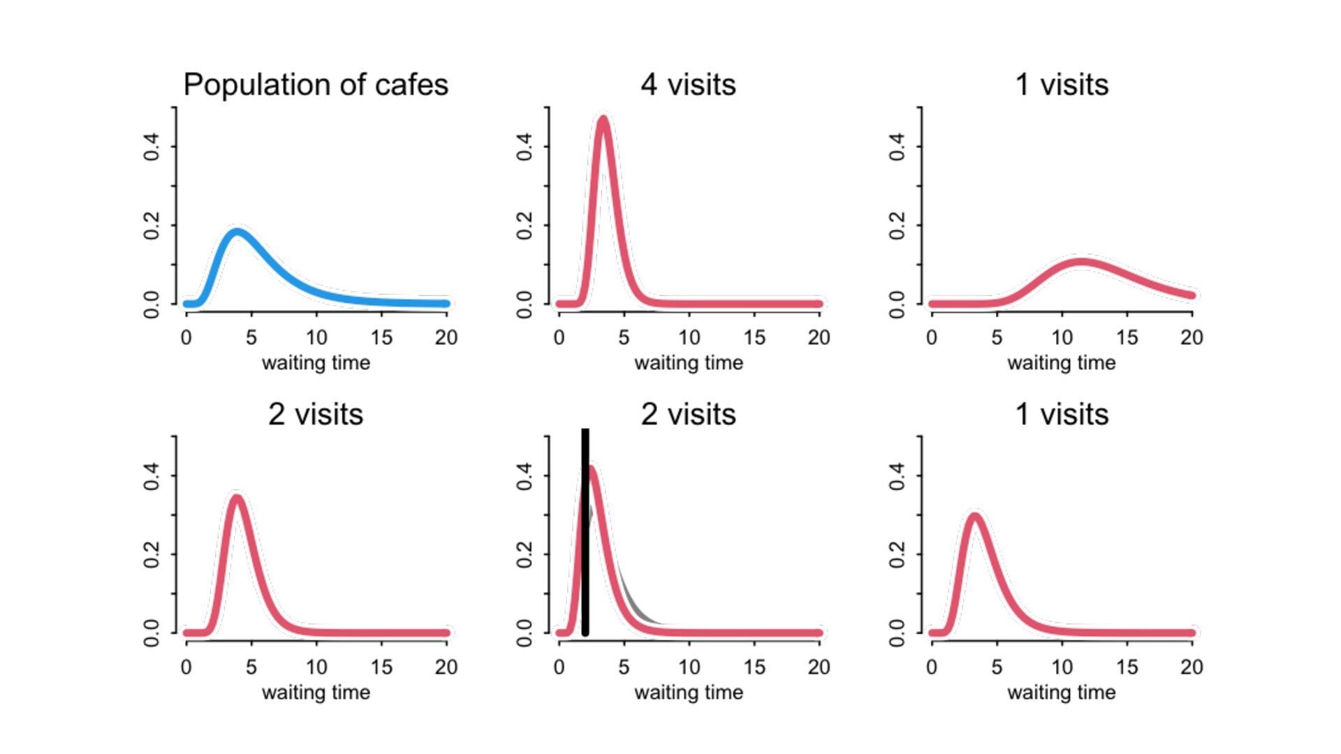
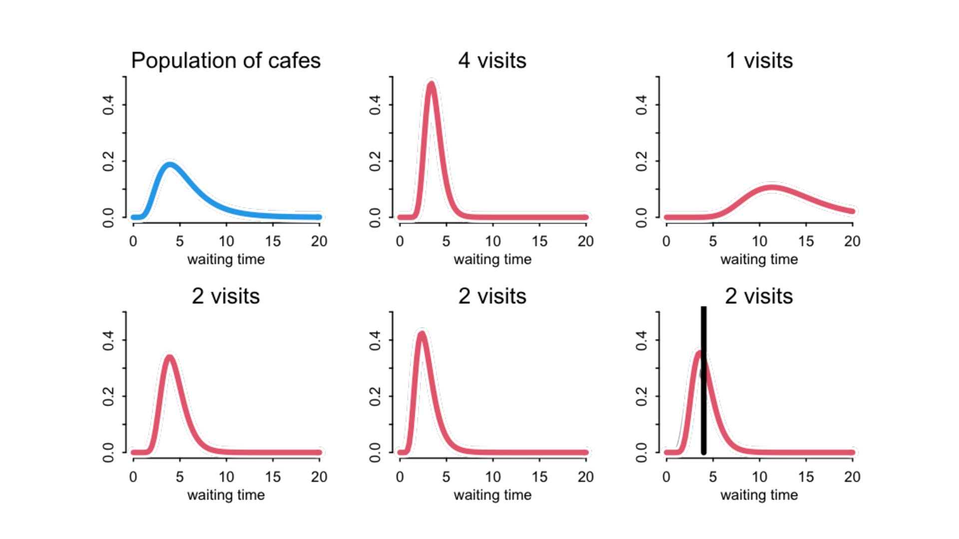
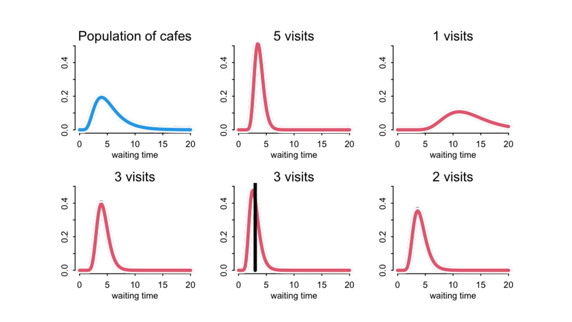
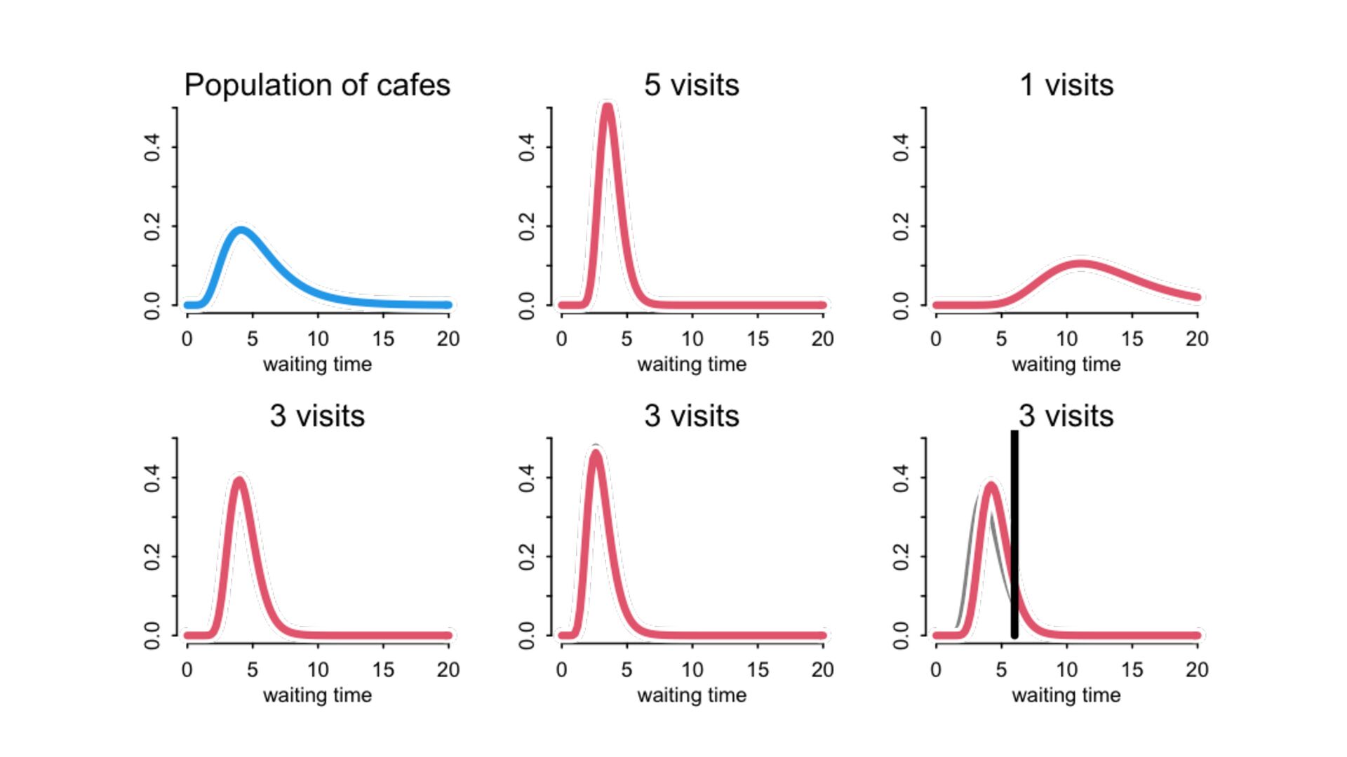
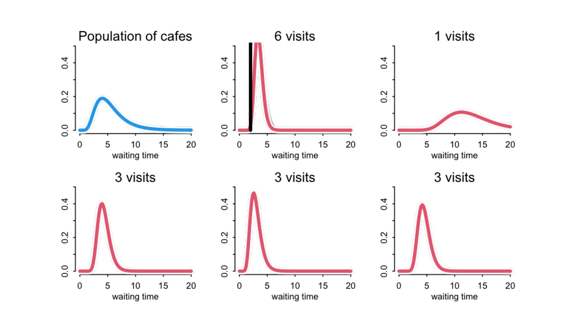
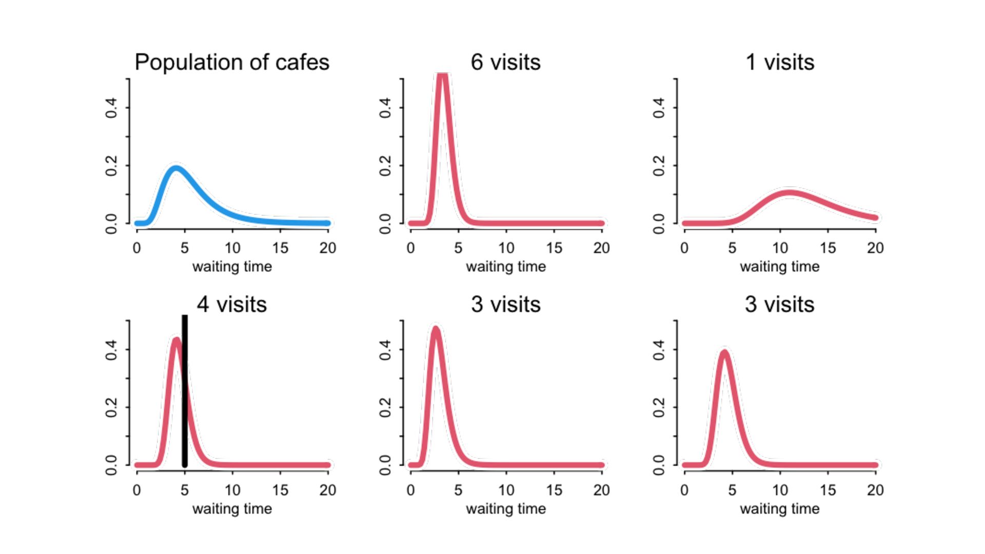
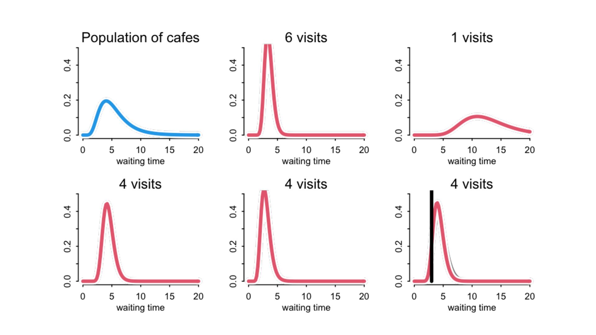
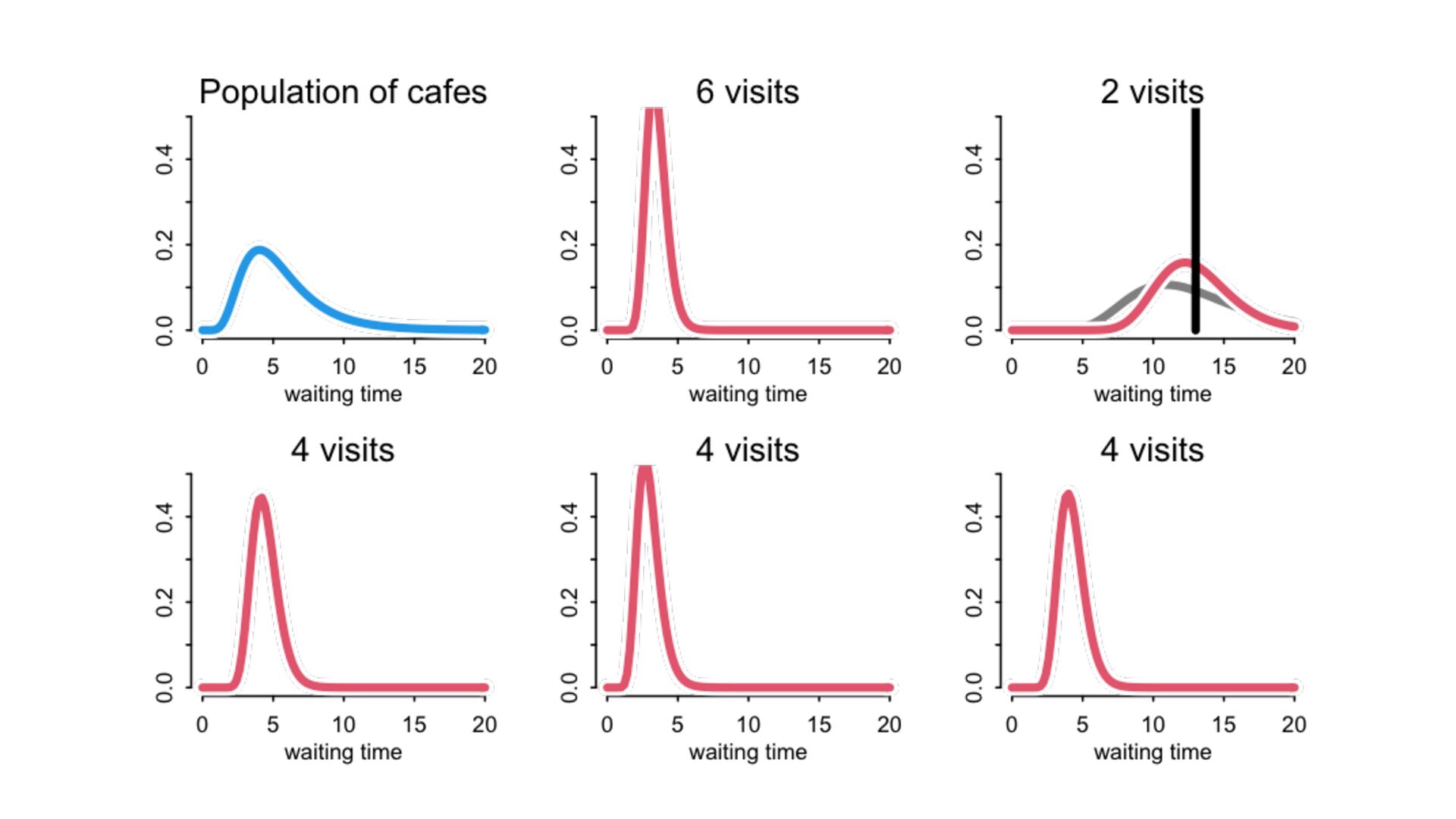
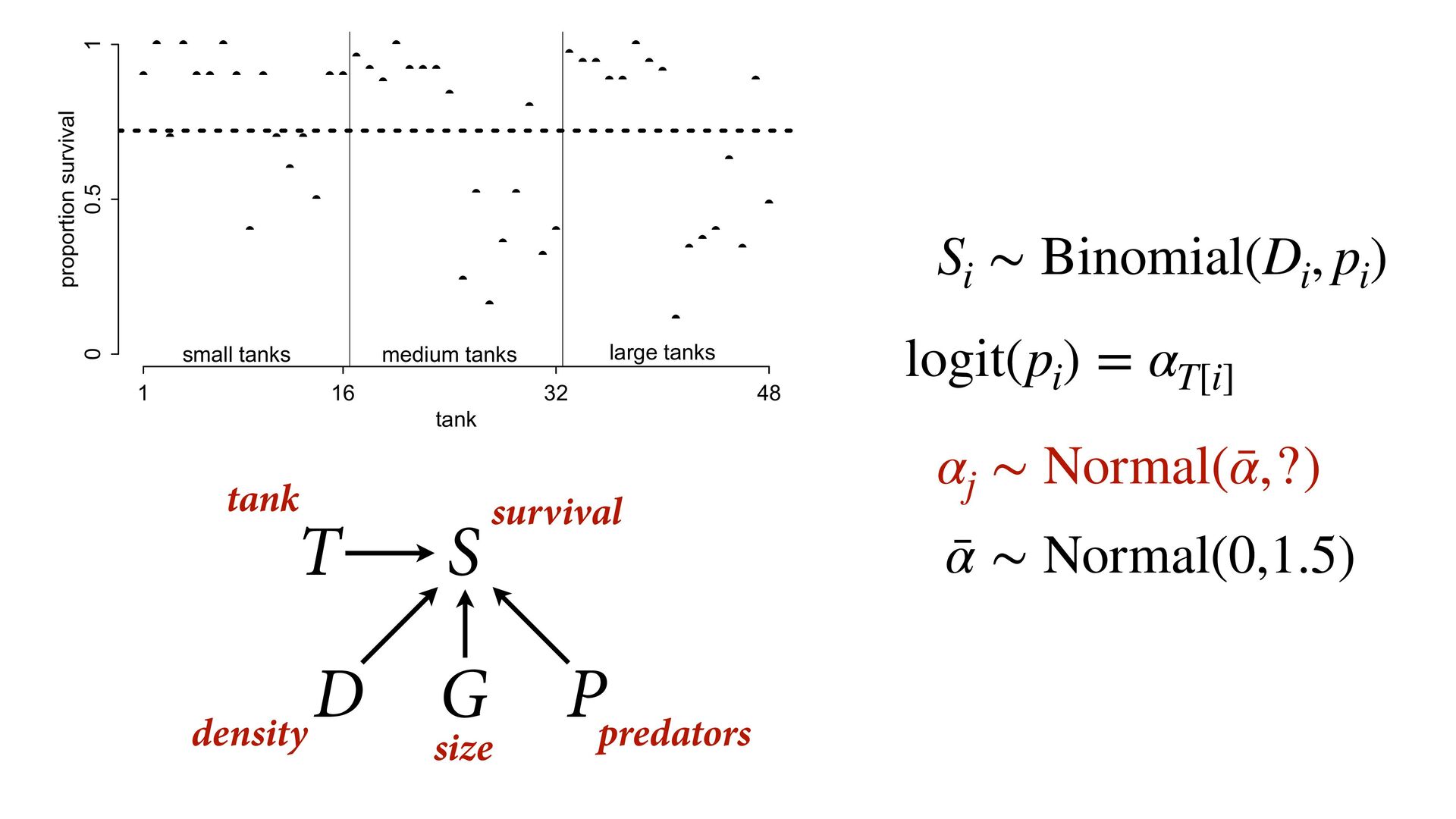
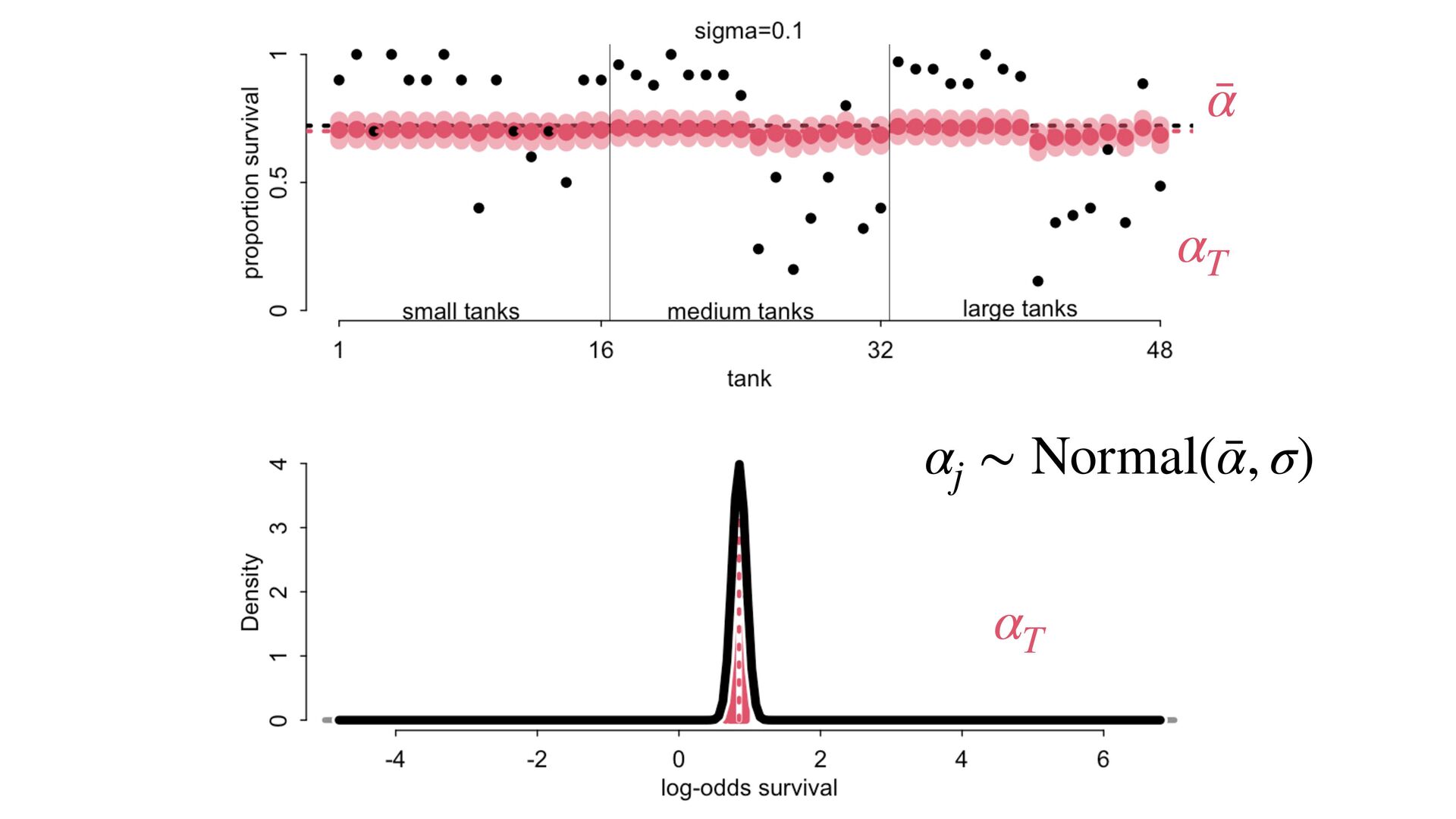
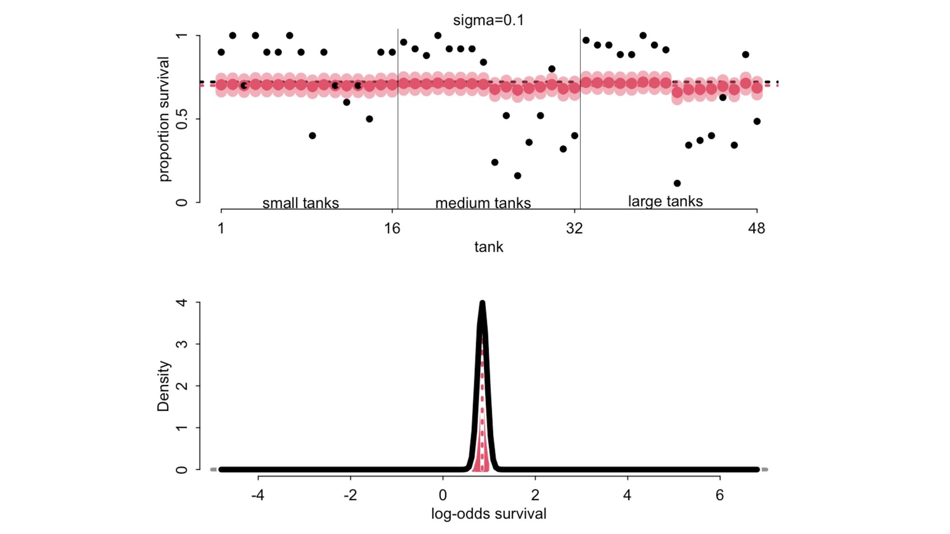
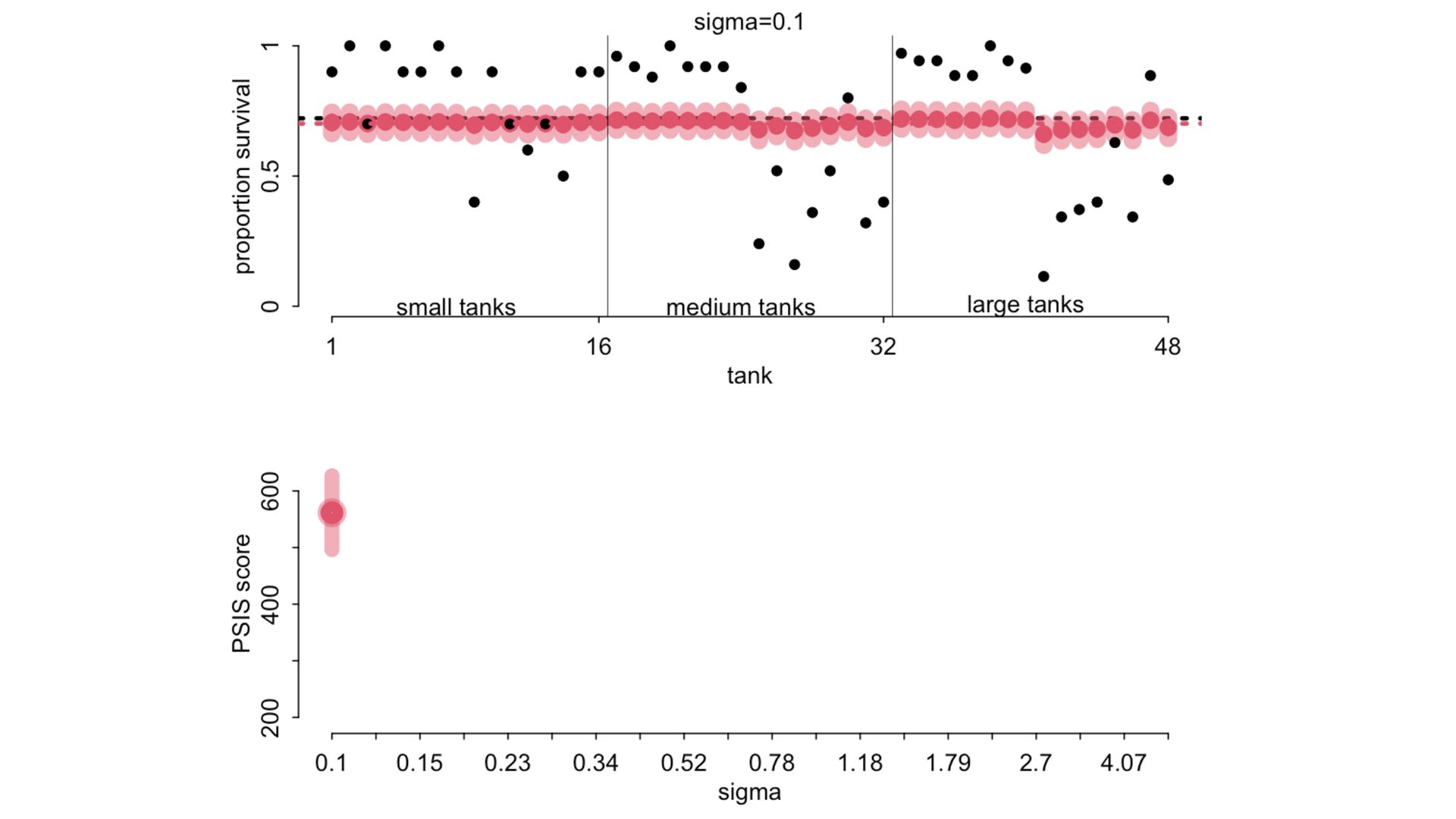
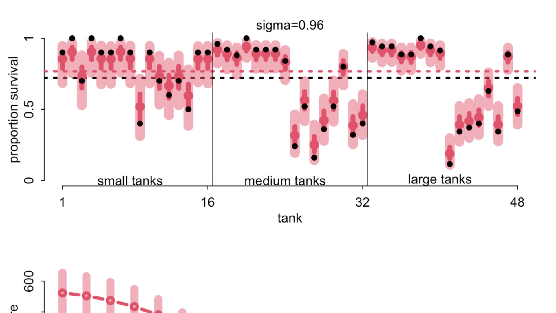
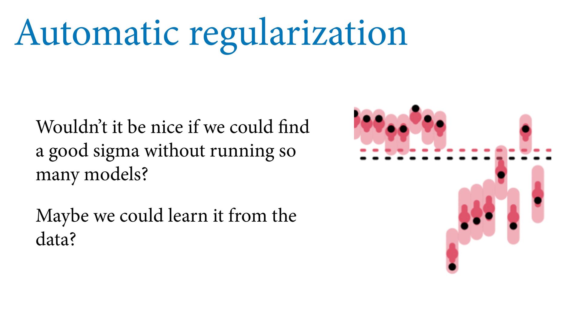
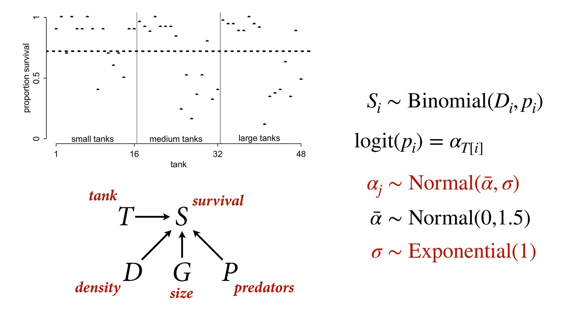
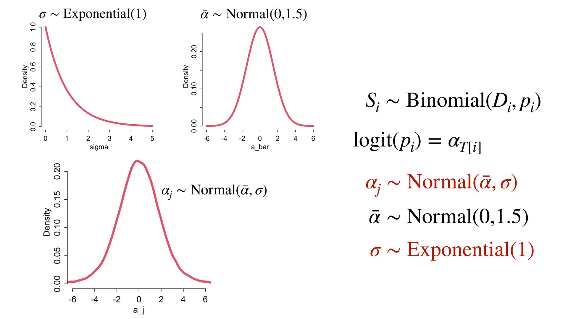
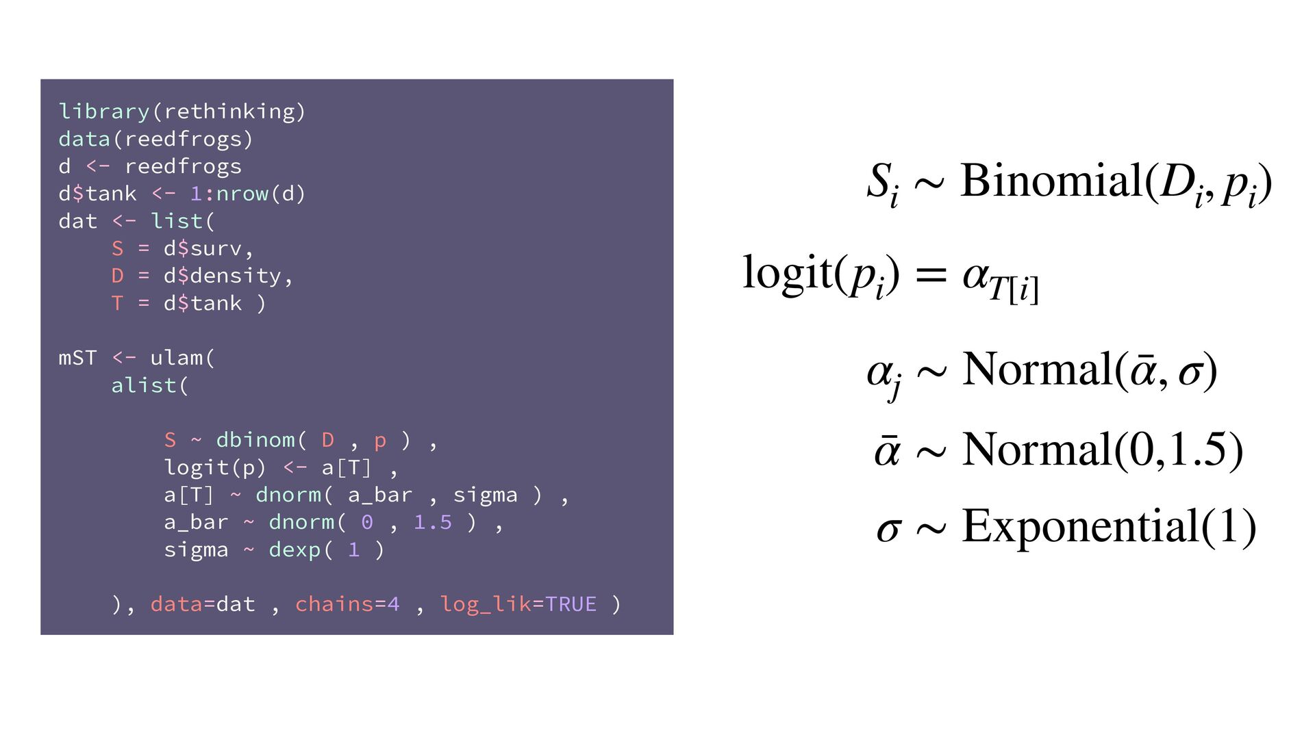
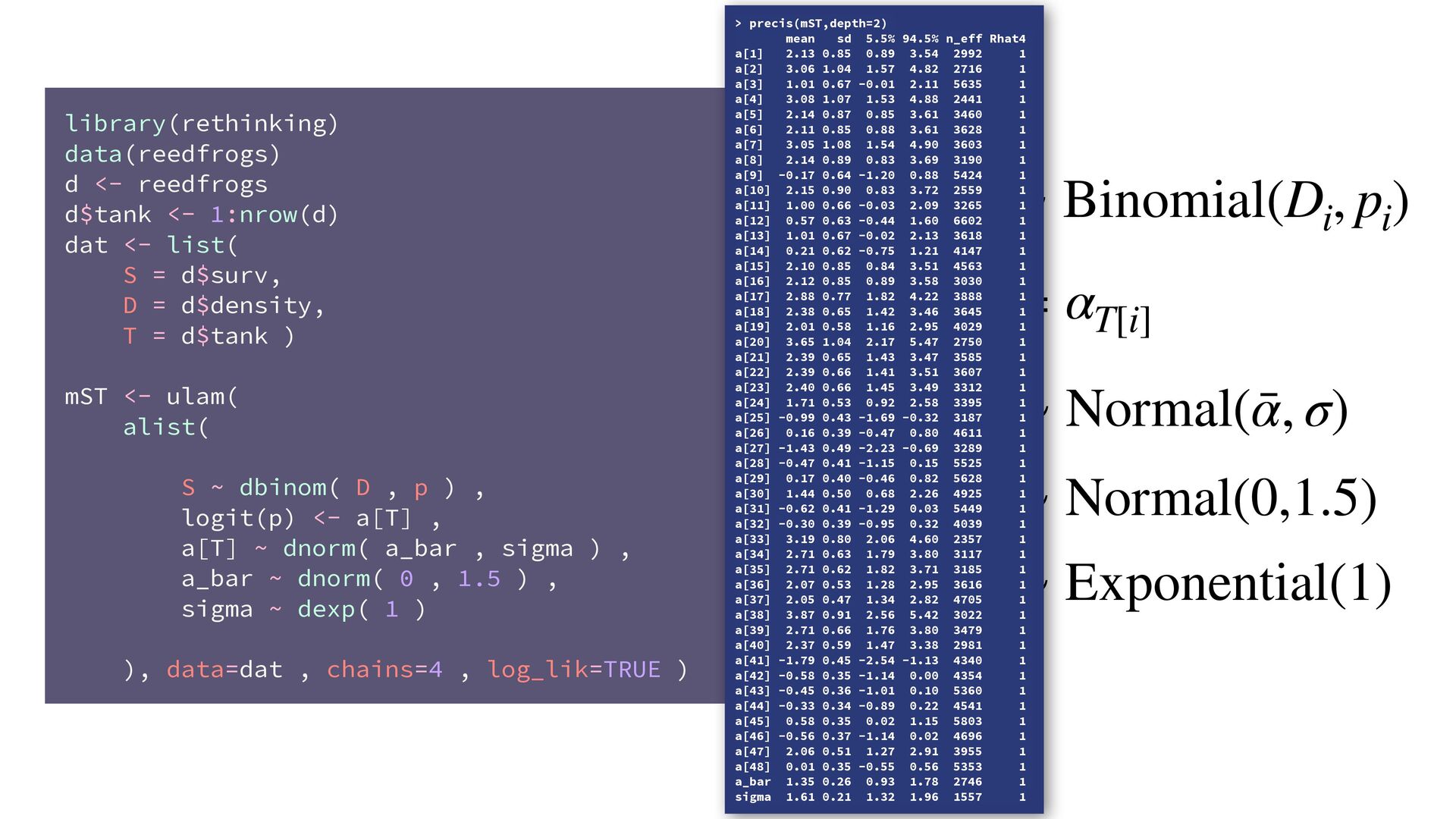
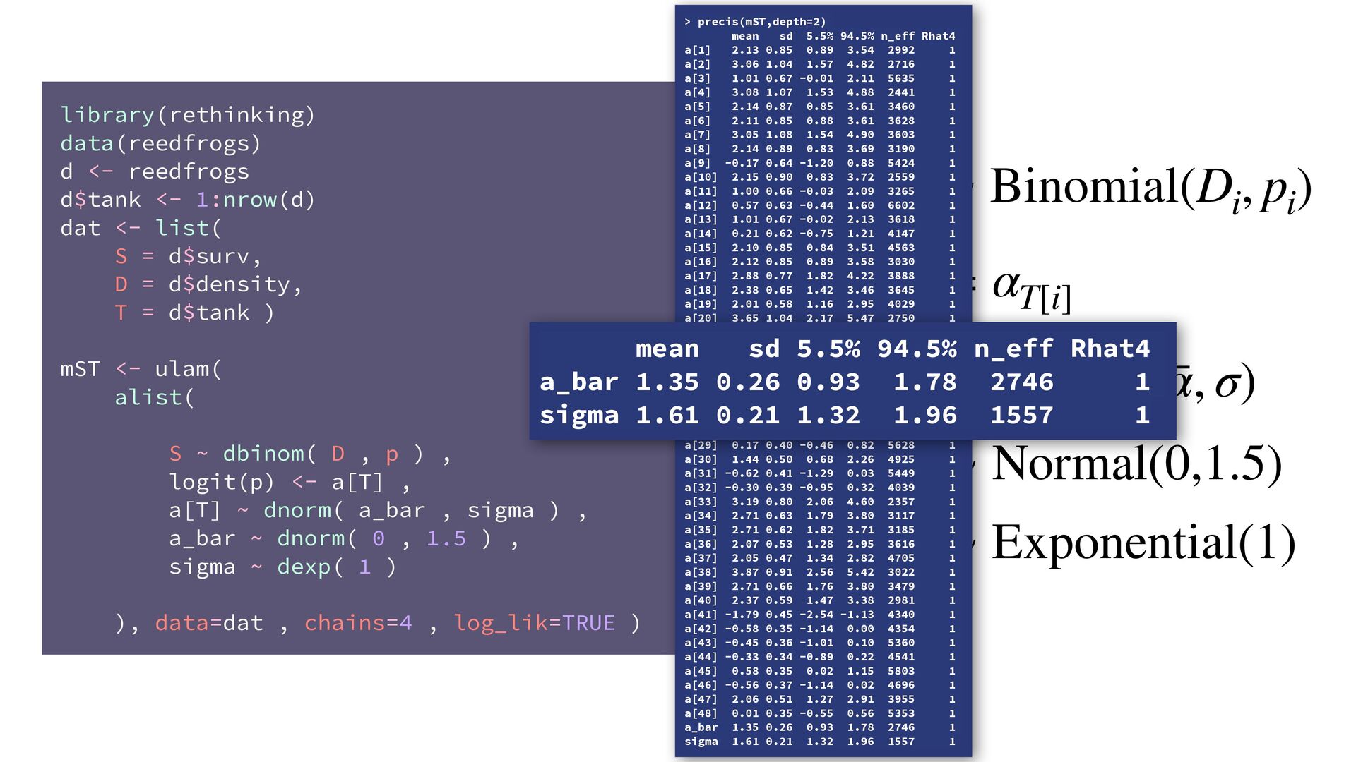
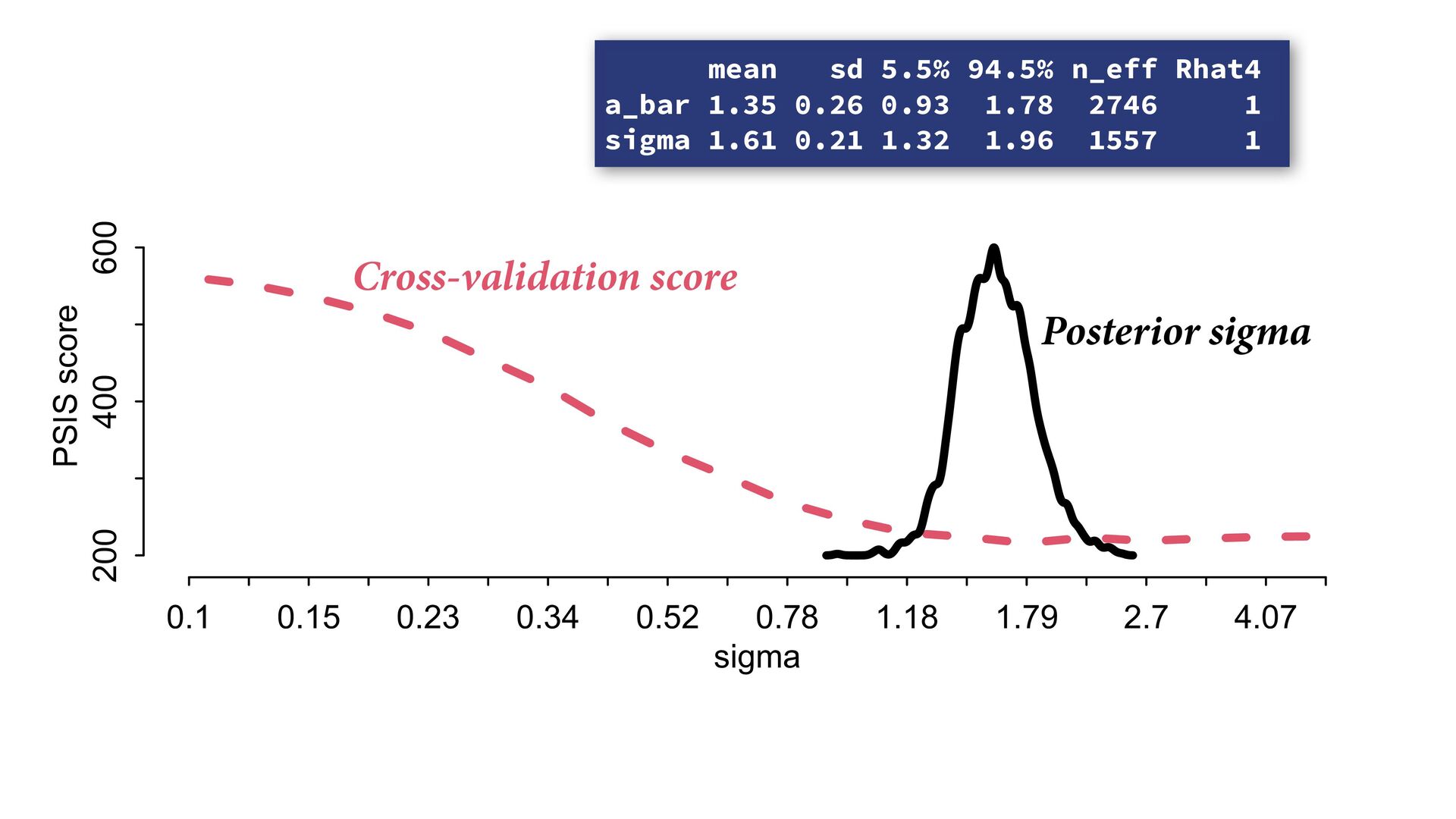
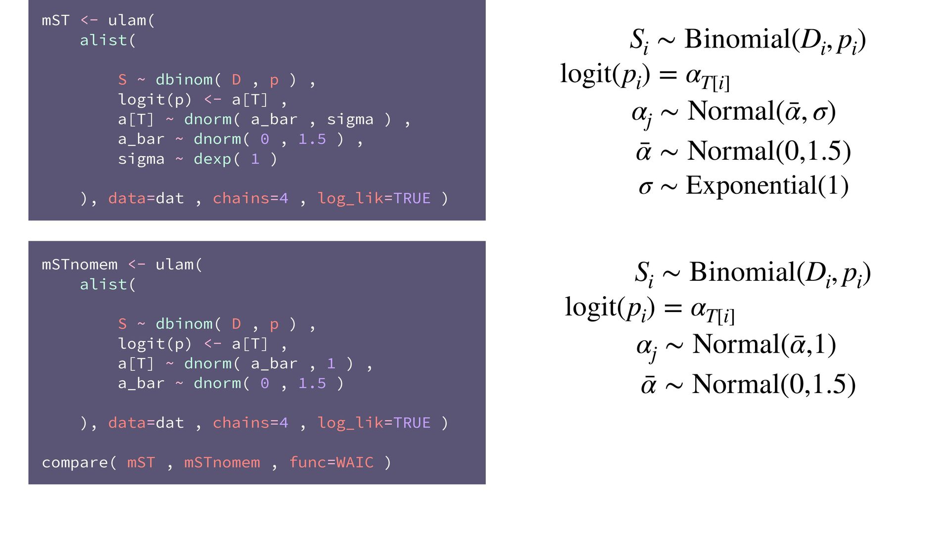
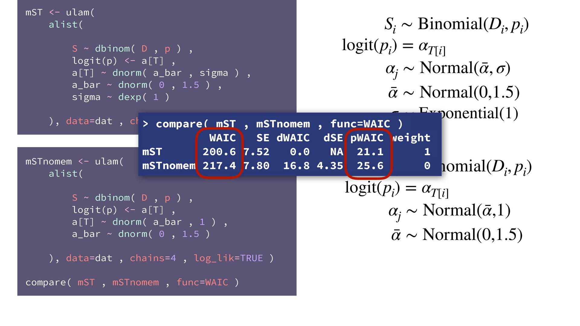
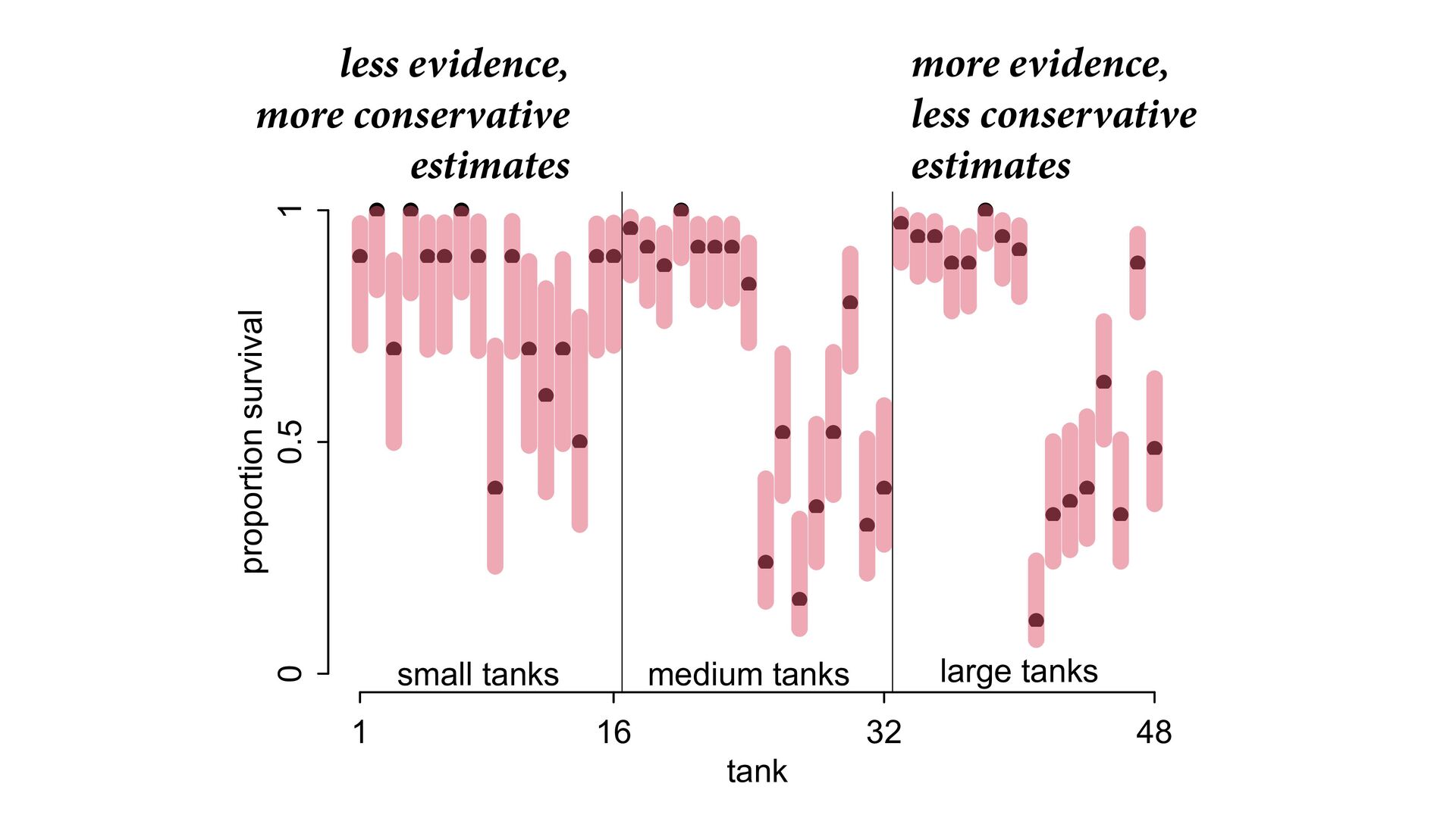
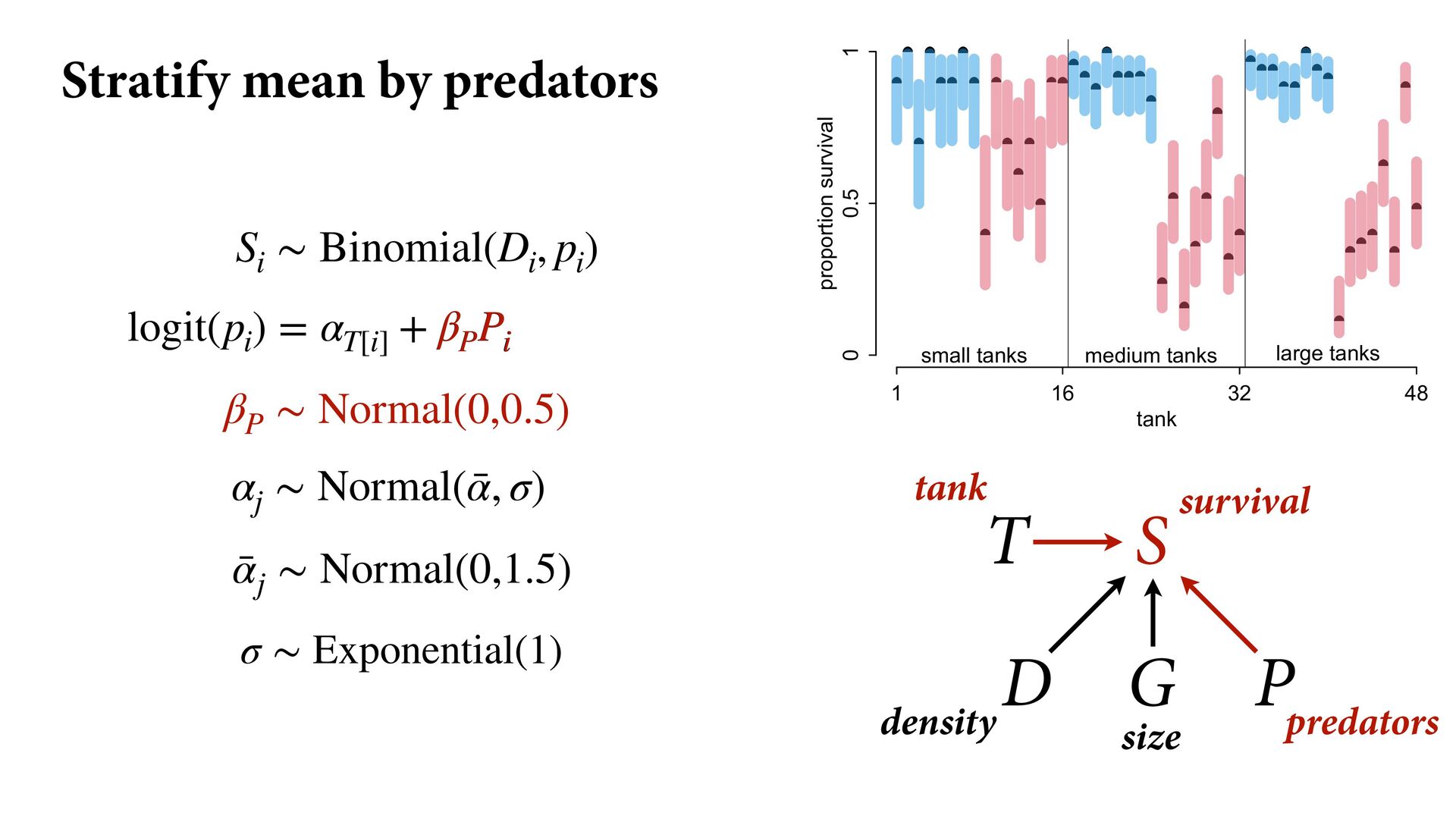
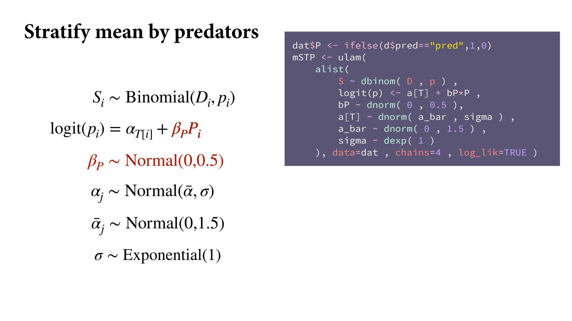
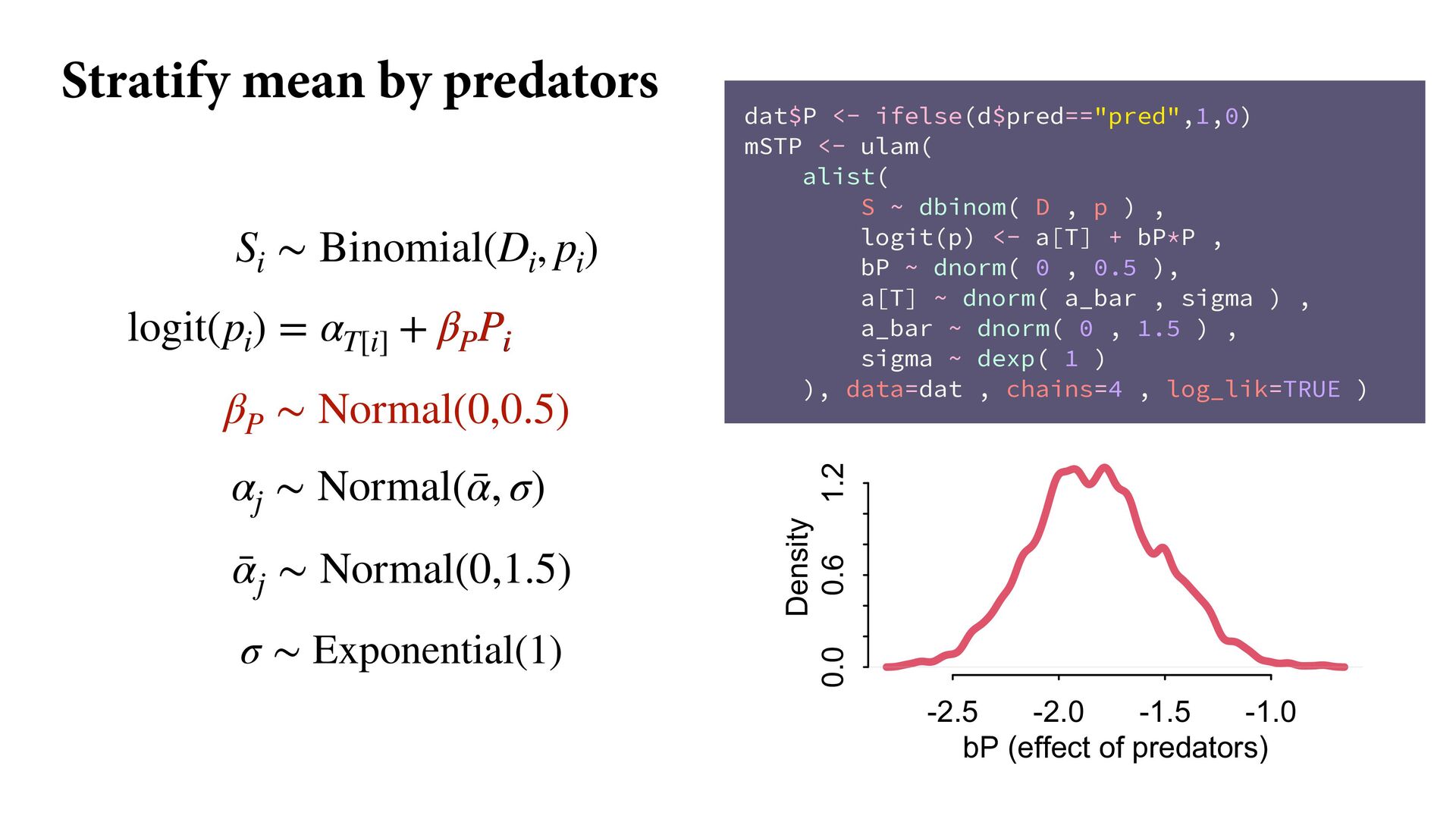
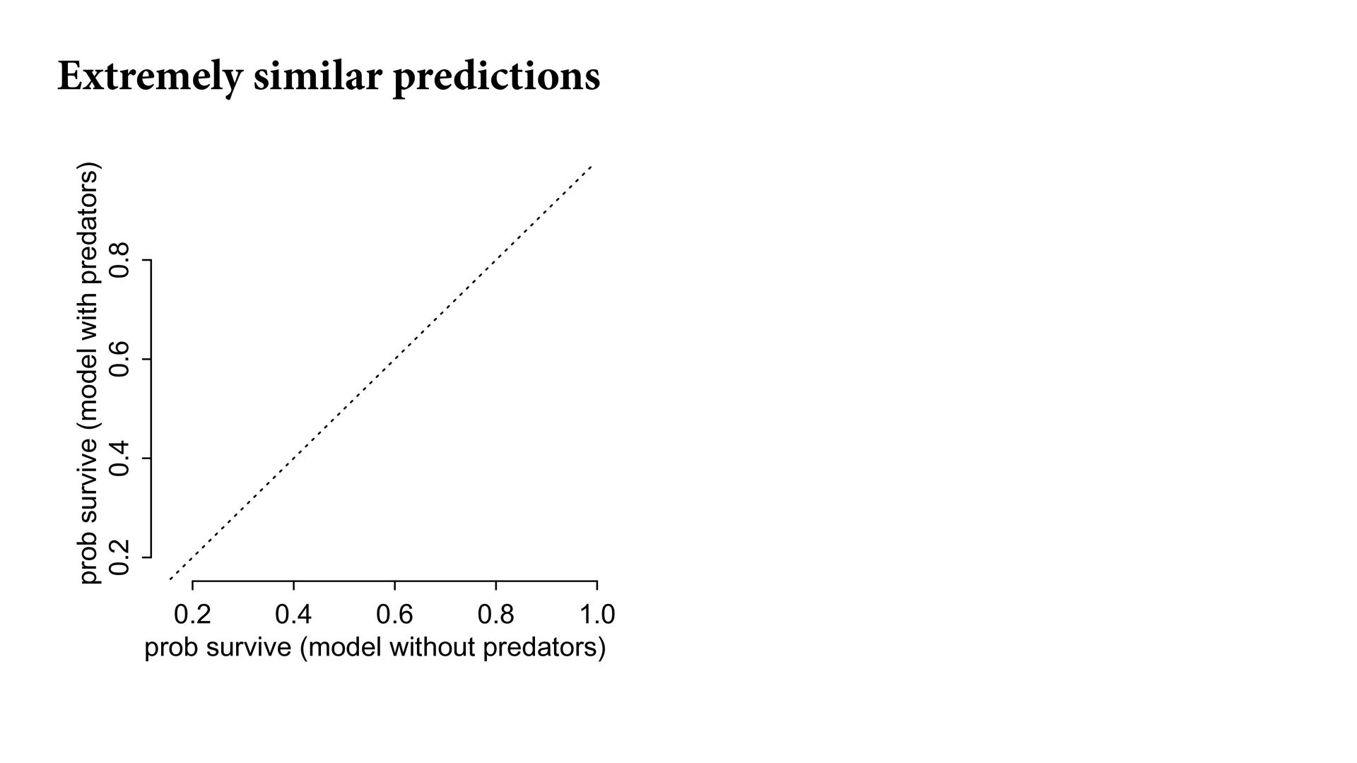
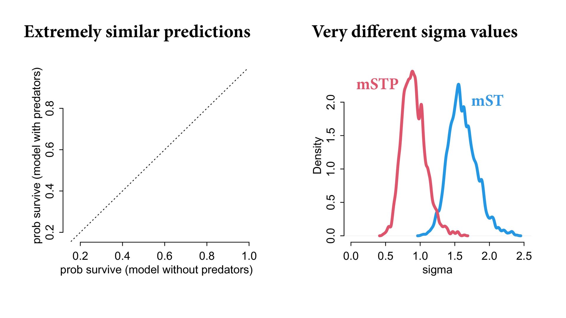
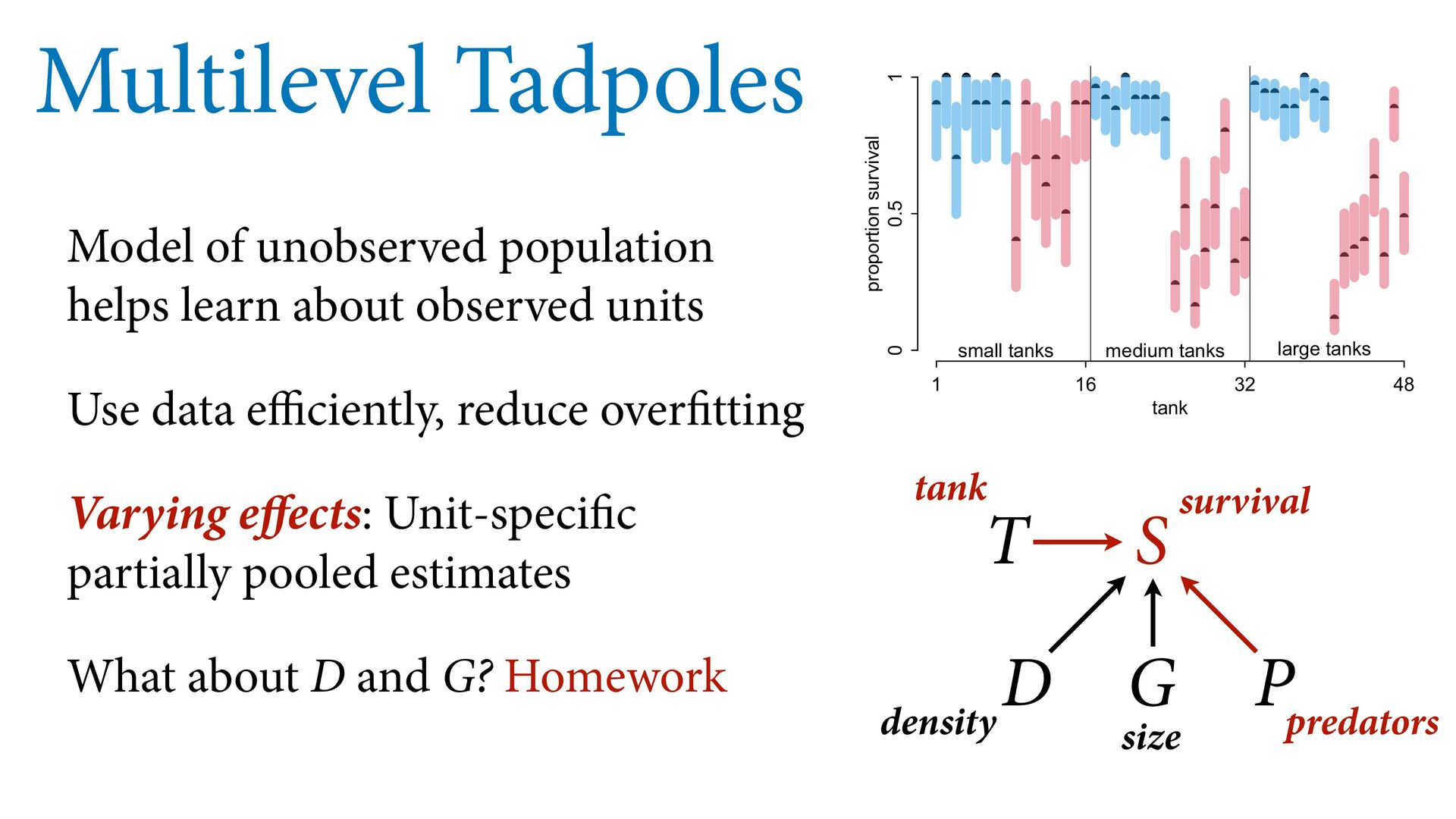
) , logit(p) <- a[T] , a[T] ~ dnorm( a_bar , 1 ) , a_bar ~ dnorm( 0 , 1.5 ) ), data=dat , chains=4 , log_lik=TRUE ) compare( mST , mSTnomem , func=WAIC ) mST <- ulam( alist( S ~ dbinom( D , p ) , logit(p) <- a[T] , a[T] ~ dnorm( a_bar , sigma ) , a_bar ~ dnorm( 0 , 1.5 ) , sigma ~ dexp( 1 ) ), data=dat , chains=4 , log_lik=TRUE ) S i ∼ Binomial(D i , p i ) logit(p i ) = α T[i] ¯ α ∼ Normal(0,1.5) α j ∼ Normal( ¯ α, σ) σ ∼ Exponential(1) S i ∼ Binomial(D i , p i ) logit(p i ) = α T[i] ¯ α ∼ Normal(0,1.5) α j ∼ Normal( ¯ α,1) > compare( mST , mSTnomem , func=WAIC ) WAIC SE dWAIC dSE pWAIC weight mST 200.6 7.52 0.0 NA 21.1 1 mSTnomem 217.4 7.80 16.8 4.35 25.6 0 Adding parameters can reduce overfitting What matters is structure, not number