Introduction to Data Science MSc lecture: A data science example

Lecture given as part of "Introduction to Data Science" MSc module at City University London, London

Transcript

1. Social research through data science: using passively-collected bikeshare datasets to study cycling behaviour Roger Beecham, gicentre.net/
2. Data Scientist: The Sexiest Job of the 21st Century Meet the people who can coax treasure out of messy, unstructured data. by Thomas H. Davenport and D.J. Patil hen Jonathan Goldman ar- rived for work in June 2006 at LinkedIn, the business networking site, the place still felt like a start-up. The com- pany had just under 8 million accounts, and the number was growing quickly as existing mem- bers invited their friends and col- leagues to join. But users weren’t seeking out connections with the people who were already on the site at the rate executives had expected. Something was apparently miss- ing in the social experience. As one LinkedIn manager put it, “It was like arriving at a conference reception and realizing you don’t know anyone. So you just stand in the corner sipping your drink—and you probably leave early.” 70  Harvard Business Review October 2012 Analytics and data science job growth
3. What makes this a data science or data- driven social research project?
4. What makes this a data science or data- driven social research project? What are the (distinct) challenges associated with doing such work?
5. What makes this a data science or data- driven social research project? What are the (distinct) challenges associated with doing such work? How can visualization techniques support this type of data analysis activity?
6. Data science implies you’re researching something: studying empirical evidence, deriving hypotheses, making claims on the quality of that evidence
7. Data science implies you’re researching something: studying empirical evidence, deriving hypotheses, making claims on the quality of that evidence But that you’re doing so with new, big and repurposed data
8. My science question: how do individuals variously cycle in big cities and what motivates or discourages that activity?
9. My science question: how do individuals variously cycle in big cities and what motivates or discourages that activity? My data question: can we use data collected passively from bikeshare schemes to answer these sorts of questions?
10. Typical research design
11. Typical research design Specify research questions and constraints Amongst London residents, what are the factors/discriminants that best explain commuting to work by bike?  
12. Typical research design Amongst London residents, what are the factors/discriminants that best explain commuting to work by bike? Define sample frame London working age/employed people, controlling for categories of age, gender, occupation, borough, distance from central London.
13. Define concepts to be measured/ collected Typical research design Amongst London residents, what are the factors/discriminants that best explain commuting to work by bike? emographic and contextual variables (cycling experience) and attitudinal variables
14. Typical research design Specify techniques Amongst London residents, what are the factors/discriminants that best explain commuting to work by bike? Outcome variable: number of commuting journeys by bike per week Independent variables: demographic, contextual, attitudinal Statement about confounders
16. Research design How, and to what extent, can the LCHS dataset be used to research on cycling behaviour? How are individual LCHS customers’ usage behaviours differentiated? How might usage behaviours be labelled? To what extent can identified behaviours be explained?
17. Datasets and (exploratory) analysis approach
18. Datasets Customers memID ###82 gender f postcode nw5 ### distance 1.3km oac cl imd 3 recency 3 frequency 4 Journeys memID oTime dTime oStation dStation ###82 18:44:26 18:50:20 61 223 ###82 11:06:24 11:15:04 62 223 ###82 22:09:24 22:23:19 94 94 ###82 20:30:36 20:46:26 94 194 ###82 19:00:17 19:04:38 94 269 ###82 14:30:38 14:34:17 94 269 ###82 07:58:09 08:02:05 94 269 Stations stationID name easting northing capacity 1 River St\nEC2 531202 182838 19 2 Phillimore Gdns\nW8 525207 179398 37 3 Christopher St\nEC2 532984 182007 32 4 St. Chad's St\nWC1 530436 182918 23 5 Sedding St\nSW1 528050 178800 27
19. Behavioural variables: Recency-Frequency segmentation and temporal clustering
20. Recency
21. Recency 1 2 3 4 5
22. Frequency
23. Frequency 1 2 3 4 5
24. Recency-Frequency segmentation frequency 808 1428 1678 3780 8898 1612 2205 3388 5086 4300 2530 3535 4454 4001 2072 4455 4647 4078 2491 920 7186 4776 2994 1233 402 recency High RF: people who use it often and have used it recently: ‘heavy users’, often commuters. Low RF: people who used it a couple of times, but then haven’t used it for a while.
25. Temporal clustering Postworkers: 13% of members 9-to-5 ers: 26% of members Anytime users: 27% of members Weekenders: 15% of members Lunchtime users: 19% of members
26. Travel time z-scores
27. Relating customer variables with space- time patterns of behaviour
29. No weighting factor
30. Weekday am Weekday pm Waterloo King’s Cross King’s Cross Waterloo
31. Exploring behaviours: gender and bikeshare usage many short journeys made within central and the City of London. For female members, however, these inter-peak journeys are highly spatially concentrated in the more leafy parts of the city – around west London and Hyde Park – and we speculate that very few might be regarded as utilitarian. By analysing the same geo-demographic subset of male and female members, then, men’s journeys become far less predictable. Women’s journeys appear, if anything, to be more regular than do men’s and, importantly, this regularity can be seen in the spatial patterns of women’s journeys. Altering the way we choose to represent journeys within our map view enables us to better articulate this point. Figure 5 shows all journeys taken by male (top) and female (bottom) members living less than 5 km from a docking station. Rather than colouring the flow lines by journey frequency, however, we colour and order journeys according to the number of unique members making them. In order to make a fairer comparison between male and female users, we control by level of usage, and select members only within the top RF segments. Figure 5. High RF men and women living <5 km from a docking station. Flows are coloured by the number of unique members making them. Background mapping uses Ordnance Survey data Crown copyright and database right 2013. Transportation Planning and Technology 93 Downloaded by [Library Services City University London] at 15:22 17 February 2015 Exploring gendered cycling behaviours within a large-scale behavioural data-set Roger Beecham* and Jo Wood Department of Computing, giCentre, City University, London, UK (Received 10 March 2013; accepted 25 July 2013) Analysing over 10 million journeys made by members of London’s Cycle Hire Scheme, we find that female customers’ usage characteristics are demonstrably different from those of male customers. Usage at weekends and within London’s parks characterises women’s journeys, whereas for men, a commuting function is more clearly identified. Some of these variations are explained by geo-demographic differences and by an atypical period of usage during the first three months after the scheme’s launch. Controlling for each of these variables brings some convergence between men and women. However, many differences are preserved. Studying the spatio-temporal context under which journeys are made, we find that women’s journeys are highly spatially structured. Even when making utilitarian cycle trips, routes that involve large, multi-lane roads are comparatively rare, and instead female cyclists preferentially select areas of the city associated with slower traffic streets and with cycle routes slightly offset from major roads. Keywords: gender and cycling behaviour; bicycle share schemes; visual analytics; behavioural data-sets 1. Introduction As access to public or shared transport systems becomes increasingly digitised, new data- sets have emerged offering opportunities to research travel behaviour in a continuous, large-scale and non-invasive way (Blythe and Bryan 2007; Froehlich, Neumann, and Oliver 2008; Kusakabe, Iryo, and Asakura 2010; Páez, Trépanier, and Morency 2011; Lathia, Ahmed, and Capra 2012). The data produced by urban bike share schemes can be regarded as a particular instance of these new data-sets. In most recent bike share schemes, data on usage are continually reported to central databases. Researchers working within data mining (Froehlich, Neumann, and Oliver 2008; Jensen et al. 2010; Borgnat et al. 2011; Lathia, Ahmed, and Capra 2012) and information visualisation (Wood, Slingsby, and Dykes 2011) have processed and then queried these data to identify patterns of usage at various spatial and temporal resolutions. Some of these works have been used by scheme operators to help overcome problems around fleet management, and by policy- makers for better understanding usage at particular docking stations. They have nevertheless been constrained by the level of detailed information made easily available (Wood, Slingsby, and Dykes 2011; Lathia, Ahmed, and Capra 2012). In many studies, data were harvested from the web, where local transport authorities publish in real-time the *Corresponding author. Email: Roger.Beecham.1@city.ac.uk Transportation Planning and Technology, 2014 Vol. 37, No. 1, 83–97, http://dx.doi.org/10.1080/03081060.2013.844903 © 2013 Taylor & Francis Downloaded by [Library Services City University London] at 15:22 17 February 2015
32. Exploring gendered usage In bicycle-friendly cities […] cycling is an inclusive, population-wide activity. […] In car-oriented cities […] the majority of cyclists are middle-aged men. [...] So strong is the association between cycling mode share and female rates of cycling that some observers have suggested that cycle-equity in cycling is an indicator of a cycling-friendly environment. Garrard, Handy & Dill (2012: 211)
33. All journeys made by men King’s Cross Waterloo Hyde Park
34. All journeys made by women King’s Cross Waterloo Hyde Park
35. Controlling for geodemographics
36. Male <5km Sep 2011-2012 Female <5km Sep 2011-2012
37. Women’s journeys remain spatially constrained - even controlling for access period, level of usage and geo-demographics
38. Male High RF <5km Sep 2011-2012 10,700 members; 1.7m journeys
39. Female High RF <5km Sep 2011-2012 3,200 members; 457,000 journeys
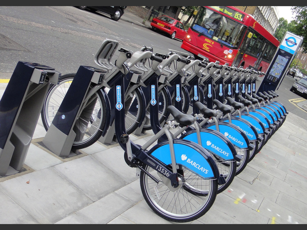
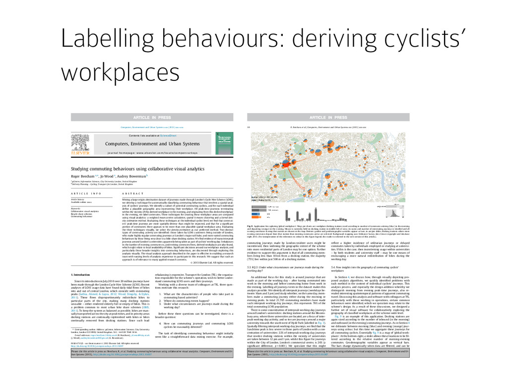
40. Studying commuting behaviours using collaborative visual analytics Roger Beecham a,⇑, Jo Wood a, Audrey Bowerman b a giCentre, Information Sciences, City University London, United Kingdom b Delivery Planning - Cycling, Transport for London, United Kingdom a r t i c l e i n f o Article history: Available online xxxx Keywords: Collaborative visual analytics Bicycle share schemes Commuting behaviour a b s t r a c t Mining a large origin–destination dataset of journeys made through London’s Cycle Hire Scheme (LCHS), we develop a technique for automatically classifying commuting behaviour that involves a spatial anal- ysis of cyclists’ journeys. We identify a subset of potential commuting cyclists, and for each individual define a plausible geographic area representing their workplace. All peak-time journeys terminating within the vicinity of this derived workplace in the morning, and originating from this derived workplace in the evening, we label commutes. Three techniques for creating these workplace areas are compared using visual analytics: a weighted mean-centres calculation, spatial k-means clustering and a kernel den- sity-estimation method. Evaluating these techniques at the individual cyclist level, we find that commut- ers’ peak-time journeys are more spatially diverse than might be expected, and that for a significant portion of commuters there appears to be more than one plausible spatial workplace area. Evaluating the three techniques visually, we select the density-estimation as our preferred method. Two distinct types of commuting activity are identified: those taken by LCHS customers living outside of London, who make highly regular commuting journeys at London’s major rail hubs; and more varied commuting behaviours by those living very close to a bike-share docking station. We find evidence of many interpeak journeys around London’s universities apparently being taken as part of cyclists’ working day. Imbalances in the number of morning commutes to, and evening commutes from, derived workplaces are also found, which might relate to local availability of bikes. Significant decisions around our workplace analysis, and particularly these broader insights into commuting behaviours, are discovered through exploring this analysis visually. The visual analysis approach described in the paper is effective in enabling a research team with varying levels of analysis experience to participate in this research. We suggest that such an approach is of relevance to many applied research contexts. Ó 2013 Elsevier Ltd. All rights reserved. 1. Introduction Since its introduction in July 2010 over 20 million journeys have been made through the London Cycle Hire Scheme (LCHS). Recent analyses of LCHS usage data have found daily tidal flows of bikes into and out of central London, which coincide with commuting peaks (Lathia, Ahmed, & Capra, 2012; Wood, Slingsby, & Dykes, 2011). These flows disproportionately redistribute bikes to particular parts of the city, making many docking stations unusable – either rendered entirely full or empty of bikes. This is a problem common to most urban bike share schemes (OBIS, 2011). To keep the system as balanced as possible, bikes are man- ually transported across the city at peak times, and in priority areas docking stations are continually replenished with bikes or bikes continually removed from docking stations. Since such load rebalancing is expensive, Transport for London (TfL), the organisa- tion responsible for the scheme’s operation, wish to better under- stand commuting LCHS users and their journeys. Working with a diverse team of colleagues at TfL, three ques- tions motivate this research: 1. What are the characteristics of people who take part in commuting based activities? 2. Where do commuting events happen? 3. Under what circumstances are journeys made during the working day? Before these three questions can be investigated, there is a broader question: 4. How can commuting journeys and commuting LCHS cyclists be reasonably detected? The task of identifying commuting behaviour might initially seem like a straightforward data mining exercise. For example, 0198-9715/$ - see front matter Ó 2013 Elsevier Ltd. All rights reserved. http://dx.doi.org/10.1016/j.compenvurbsys.2013.10.007 ⇑ Corresponding author. Address: giCentre, Information Sciences, City University London, London EC1V0HB, United Kingdom. Tel.: +44 020 7040 3914. E-mail addresses: roger.beecham.1@city.ac.uk (R. 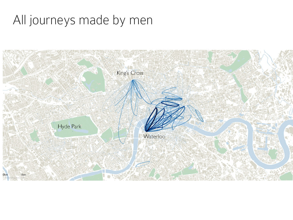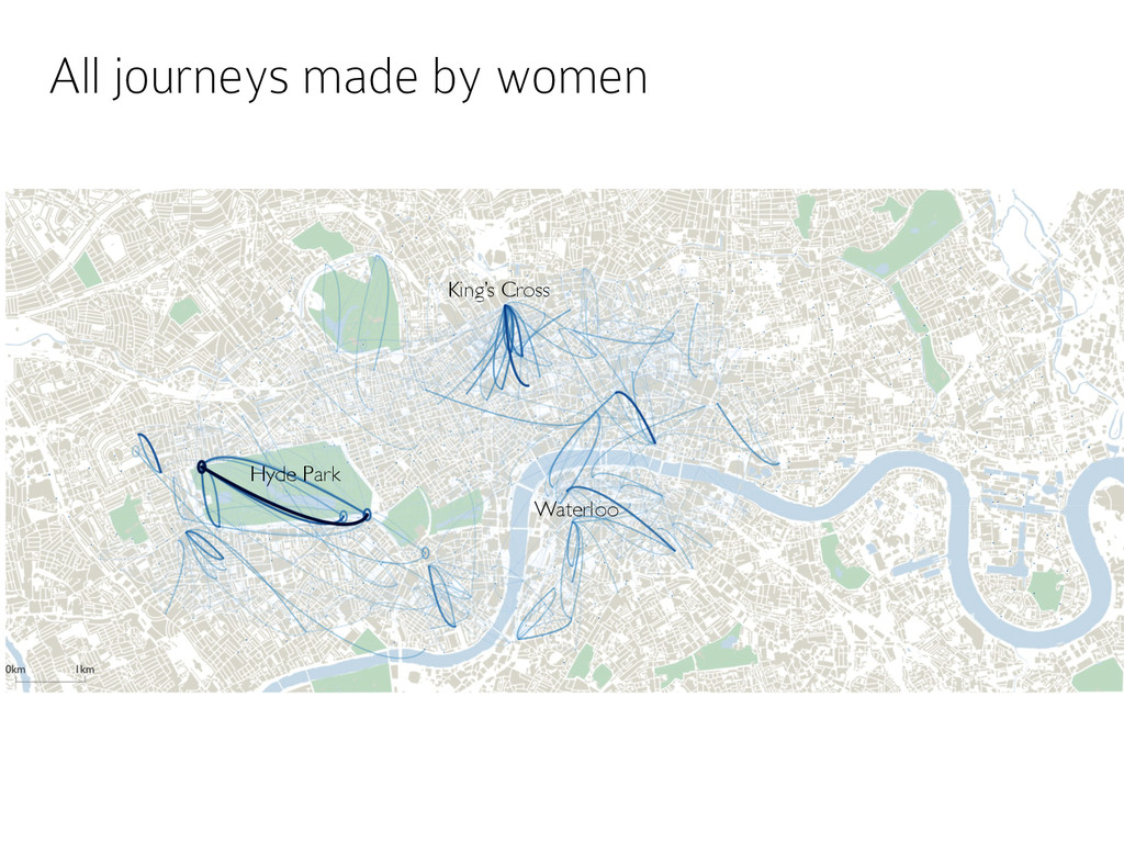Beecham), j.d.wood@city.ac.uk (J. Wood), audreybowerman@tfl.gov.uk (A. Bowerman). Computers, Environment and Urban Systems xxx (2013) xxx–xxx Contents lists available at ScienceDirect Computers, Environment and Urban Systems journal homepage: www.elsevier.com/locate/compenvurbsys Please cite this article in press as: Beecham, R., et al. Studying commuting behaviours using collaborative visual analytics. Computers, Environment and Ur- ban Systems (2013), http://dx.doi.org/10.1016/j.compenvurbsys.2013.10.007 commuting journeys made by London-resident users might be incentivised, then widening the geographic extent of the scheme into more residential parts of London may be one option. Further evidence to support this argument is that of all commuting mem- bers living less than 10 km from a docking station, the majority (75%) live within just 500 m of a docking station. 5.3. RQ 3: Under what circumstances are journeys made during the working day? An additional focus for this study is around journeys that are made as part of the working day – after having commuted into work in the morning and before commuting home from work in the evening. Labelling all journey events in the dataset makes this analysis possible. We identify all interpeak journeys (weekdays be- tween 10am and 3 pm) and study whether, on the same day, mem- bers make a commuting journey either during the morning or evening peaks. In total 21,765 commuting members have made such interpeak working-day journeys; this represents 78% of the total commuting LCHS population. There is some concentration of interpeak working-day journeys around London’s universities: docking stations around the Blooms- bury area, where three universities are located, are a focus of inter- peak working-day activity, and so too are journeys around a major university towards the south west of Hyde Park (labelled in Fig. 3). Spatially filtering interpeak working-day journeys, we find that the lunchtime peak is less severe in those parts of London with a con- centration of universities: 22% of interpeak working-day journeys that involve docking stations within the vicinity of universities are taken between 12 pm and 1 pm, whilst this figure for journeys within the City of London, London’s commercial centre, is 26% (a significant difference, p < 0.001). We speculate that this might reflect a higher incidence of utilitarian journeys or delayed commutes taken by individuals employed or studying at universi- ties. If this is the case, then incentivising usage within universities – by both students and university staff – may be one means of encouraging a more natural redistribution of bikes during the working day. 5.4. New insights into the geography of commuting cyclists’ workplaces In Section 4, we discuss how, through visually depicting pro- posed analysis algorithms, we quickly identified problems with each method in the context of individual cyclists’ journeys. This analysis process, and especially the design addition whereby we distinguish morning from evening peak-time journeys, also re- vealed interesting spatiotemporal patterns of apparent commuting travel. Discussing this analysis and software with colleagues at TfL, particularly with those working in operations, certain common behaviours were identified, which we speculate may relate to the scheme’s design. As a result of these discussions, we designed a further set of visual software for collaboratively exploring the geography of classified workplaces at the scheme-wide level. Fig. 9 is an example of this application. Docking stations are again sized according to the number of inbound (in the morning) and outbound (in the evening) commuting journeys. As in Section 4 we delineate between morning (blue) and evening (orange) jour- neys using colour, but this time we aggregate these journeys for all commuting cyclists. Essentially fig. 9 is a map of ‘global work- places’. At the bottom-right, a slider allows these locations to be fil- tered according to the relative number of morning-evening commutes. Geodemographic variables appear as vertical bars. The bars change dynamically when data are filtered, and can be Fig. 9. Application for exploring ‘global workplaces’. Map: pie charts are workplace docking stations sized according to number of commutes arriving (blue) in the morning and departing (orange) in the evening. Mouse is currently held on docking station in middle left of view; its name and number of commuting journeys is labelled and all evening commutes leaving that station are drawn on the map. Bottom: gender and geodemographic variables appear as bars; in am/pm slider, docking stations where more evening commutes depart from that station than morning commutes arrive are selected. Background mapping uses Ordnance Survey data Crown copyright and database right 2013. (For interpretation of the references to colour in this figure legend, the reader is referred to the web version of this article.). 10 R. Beecham et al. / Computers, Environment and Urban Systems xxx (2013) xxx–xxx Please cite this article in press as: Beecham, R., et al. Studying commuting behaviours using collaborative visual analytics. Computers, Environment and Ur- ban Systems (2013), http://dx.doi.org/10.1016/j.compenvurbsys.2013.10.007 Labelling behaviours: deriving cyclists’ workplaces
41. Labelling behaviours: identifying group cycling Characterising group-cycling journeys using interactive graphics Roger Beecham ⇑, Jo Wood giCentre, Department of Computer Science, City University London, United Kingdom a r t i c l e i n f o Article history: Received 21 June 2013 Received in revised form 24 December 2013 Accepted 11 March 2014 Available online 18 April 2014 Keywords: Bikeshare schemes Bicycling behaviour Visual analytics a b s t r a c t The group-cycling behaviours of over 16,000 members of the London Cycle Hire Scheme (LCHS), a large public bikeshare system, are identified and analysed. Group jour- neys are defined as trips made by two or more cyclists together in space and time. Detailed insights into group-cycling behaviour are generated using specifically designed visualiza- tion software. We find that in many respects group-cycle journeys fit an expected pattern of discretionary activity: group journeys are more likely at weekends, late evenings and lunchtimes; they generally take place within more pleasant parts of the city; and between individuals apparently known to each other. A separate set of group activity is found, however, that coincides with commuting peaks and that appears to be imposed onto LCHS users by the scheme’s design. Studying the characteristics of individuals making group journeys, we identify a group of less experienced LCHS cyclists that appear to make more spatially extensive journeys than they would do normally while cycling with others; and that female cyclists are more likely to make late evening journeys when cycling in groups. For 20% of group cyclists, the first journey ever made through the LCHS was a group jour- ney; this is particularly surprising since just 9% of all group cyclists’ journeys are group journeys. Moreover, we find that women are very significantly (p < 0.001) overrepresented amongst these ‘first time group cyclists’. Studying the bikeshare cyclists, or bike share ‘friends’, that individuals make ‘first time group journeys’ with, we find a significantly high incidence (p < 0.001) of group journeys being made with friends of the opposite gender, and for a very large proportion (55%) of members these first ever journeys are made with a friend that shares the same postcode. A substantial insight, then, is that group cycling appears to be a means through which early LCHS usage is initiated. Ó 2014 Elsevier Ltd. All rights reserved. 1. Introduction The many economic, health-related and environmental benefits of cycling have precipitated a growing academic interest in understanding cycling behaviour, and particularly the factors that motivate and discourage cycling within cities (Pucher and Buehler, 2012). Here, researchers have identified distinct cycling behaviours related to factors such as gender and social demographics (Anable et al., 2010; Heesch et al., 2012), individuals’ life stages (Bonham and Wilson, 2012; Pooley et al., 2011), more obvious weather-related variables (Thomas et al., 2008) and the nature and provision of cycling infrastructure (Garrard et al., 2008; Dill and Gliebe, 2008; Tilahun et al., 2007). Relatively little research, either observational or attitudinal, http://dx.doi.org/10.1016/j.trc.2014.03.007 0968-090X/Ó 2014 Elsevier Ltd. All rights reserved. ⇑ Corresponding author. Address: giCentre, Department of Computer Science, City University London, College Building, Northampton Square, City University London, London EC1V 0HB, United Kingdom. E-mail addresses: Roger.Beecham.1@city.ac.uk (R. Beecham), J.D.Wood@city.ac.uk (J. Wood). Transportation Research Part C 47 (2014) 194–206 Contents lists available at ScienceDirect Transportation Research Part C journal homepage: www.elsevier.com/locate/trc scheme users living relatively close to a LCHS docking station, and it perhaps makes sense that those making group journeys later in the evening fit this profile. We also find, however, that women are significantly overrepresented (p < 0.001) amongst the group members who make these late evening journeys. Whilst 28% of all group cyclists are women, 33% of group cyclists making late evening group journeys are women. This is particularly surprising as when we look at all journeys (both group Fig. 6. Temporal and spatial views of group journeys by cluster membership. Temporal view: all journeys in grey, group journeys in blue. Map view: non- group journeys are blue, group journeys are red. Journey lines are weighted by the number of members making journeys. Since group cyclists represent just 20% of LCHS members, if we were to use the same colour scale to weight group journeys as non-group journeys it would be very difficult make a comparison; non-group journeys would appear very light and transparent in colour. To enable better comparison, colour weightings for group and non- group journeys are therefore scaled independently. (For interpretation of the references to colour in this figure legend, the reader is referred to the web version of this article.) Background mapping uses Ordnance Survey data Crown copyright and database right 2014. 202 R. Beecham, J. Wood / Transportation Research Part C 47 (2014) 194–206
42. Explaining behaviours: deriving likely routes and investigating likely route choice
44. Conflating actual with estimated routes?
45. Research questions
46. Research questions RQ1. Which bridges are most likely to be used by men and women?
47. Research questions RQ1. Which bridges are most likely to be used by men and women? RQ2. To what extent are these bridges crossed equally in either direction (northbound and southbound)?
48. Research questions RQ1. Which bridges are most likely to be used by men and women? RQ2. To what extent are these bridges crossed equally in either direction (northbound and southbound)? RQ3. Are journeys that involve a river crossing generally more demanding than other journeys made between LCHS docking stations?
49. London Bridge! Southwark Bridge! Blackfriars Bridge! Waterloo Bridge! Westminster Bridge! Lambeth Bridge! Vauxhall Bridge!
51. Counted journeys over ‘suggested’ bridges
52. Men’s and women’s usage of bridges
53. Geography of men’s and women’s workplaces
54. Men’s and women’s usage of bridges
55. Men’s and women’s usage of bridges
56. Are (suggested) cycled journeys over certain bridges more demanding than others? !
57. Are (suggested) cycled journeys over certain bridges more demanding than others? !
58. Are (suggested) cycled journeys over certain bridges more demanding than others? !
59. Discussion points Data-driven analysis approach: explore, label and possibly explain behaviours
60. Discussion points Data-driven analysis approach: explore, label and possibly explain behaviours Generalising findings: sample and measurement validity with passively collected data
61. Discussion points Data-driven analysis approach: explore, label and possibly explain behaviours Generalising findings: sample and measurement validity with passively collected data The role of visualization …
62. Exploratory vis enabled us to identify structure and generate findings early – useful in speculative analysis projects where you’re repurposing a dataset Arguments on the role of visualization
63. Arguments on the role of visualization Chauffeured analysis helped with engaging domain experts and subsequently specifying better research questions/hypotheses … (and writing better papers?)
64. Arguments on the role of visualization Visual approach might have allowed us to find out things that we couldn’t have found out using other techniques
65. Arguments on the role of visualization But how do we make or articulate research claims from findings identified through visual inspection (and using repurposed data)?  
66. Graphical Inference for Infovis Hadley Wickham, Dianne Cook, Heike Hofmann, and Andreas Buja Fig. 1. One of these plots doesn’t belong. These six plots show choropleth maps of cancer deaths in Texas, where darker colors = more deaths. Can you spot which of the six plots is made from a real dataset and not simulated under the null hypothesis of spatial independence? If so, you’ve provided formal statistical evidence that deaths from cancer have spatial dependence. See Section 8 for the answer. Abstract— How do we know if what we see is really there? When visualizing data, how do we avoid falling into the trap of apophenia where we see patterns in random noise? Traditionally, infovis has been concerned with discovering new relationships, and statistics with preventing spurious relationships from being reported. We pull these opposing poles closer with two new techniques for rigorous statistical inference of visual discoveries. The “Rorschach” helps the analyst calibrate their understanding of uncertainty and the “line- up” provides a protocol for assessing the significance of visual discoveries, protecting against the discovery of spurious structure. Index Terms—Statistics, visual testing, permutation tests, null hypotheses, data plots. 1 INTRODUCTION What is the role of statistics in infovis? In this paper we try and an- swer that question by framing the answer as a compromise between curiosity and skepticism. Infovis provides tools to uncover new rela- graphic plates of actual galaxies. This was a particularly impressive achievement for its time: models had to be simulated based on tables of random values and plots drawn by hand. As personal computers be- 973 IEEE TRANSACTIONS ON VISUALIZATION AND COMPUTER GRAPHICS, VOL. 16, NO. 6, NOVEMBER/DECEMBER 2010
67. Wickham et al. (2010) Graphical Inference  
68. Roger.beecham.1@city.ac.uk   Questions