Environmental turnover predicts plant species richness & turnover - Comparing the Greater Cape Floristic Region & the Southwest Australia Floristic Region

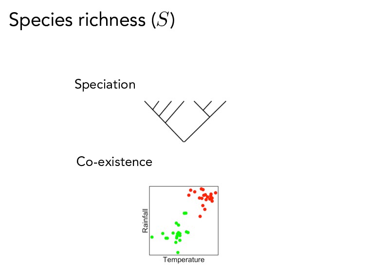
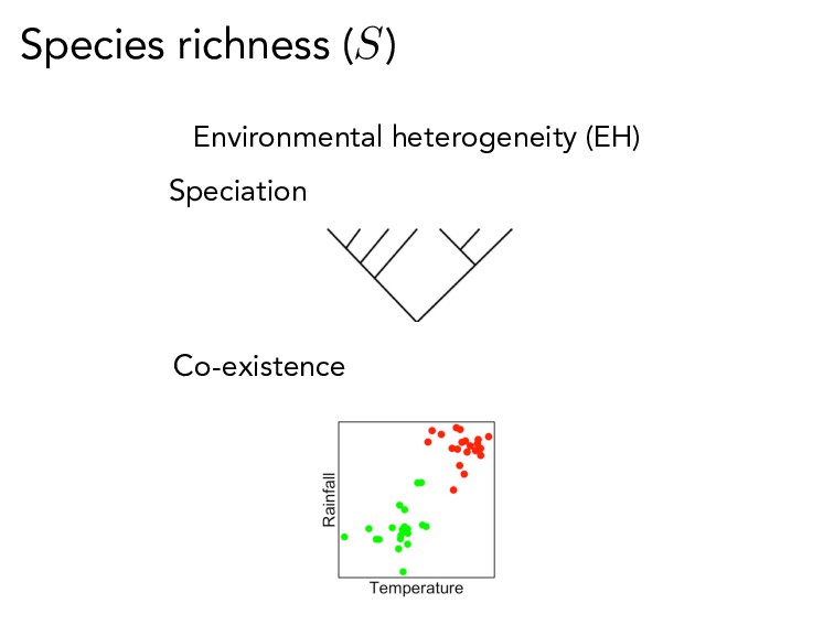
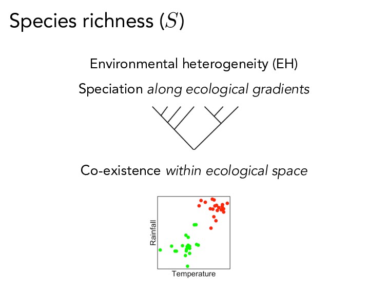
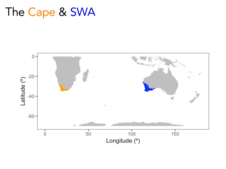
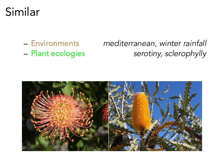
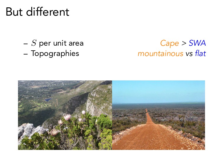
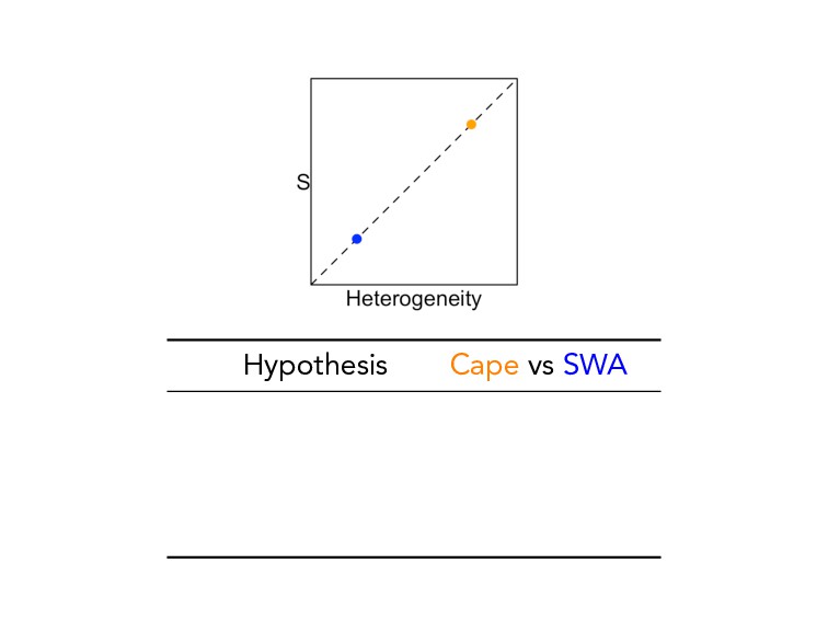
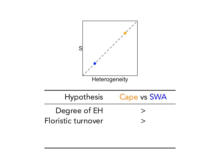
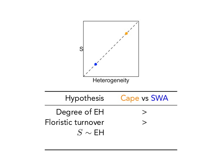
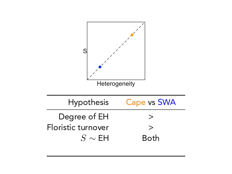
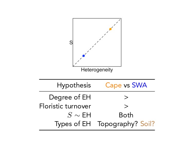
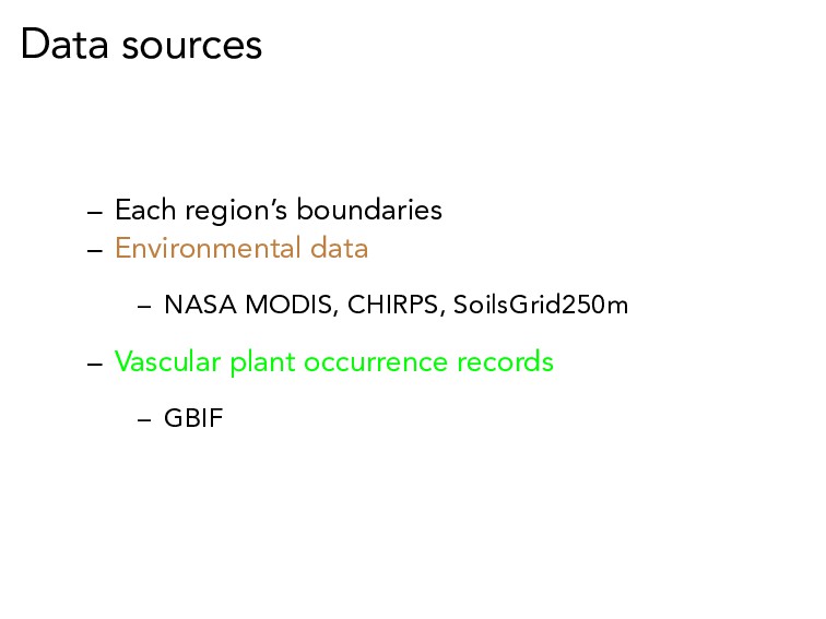
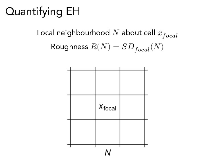
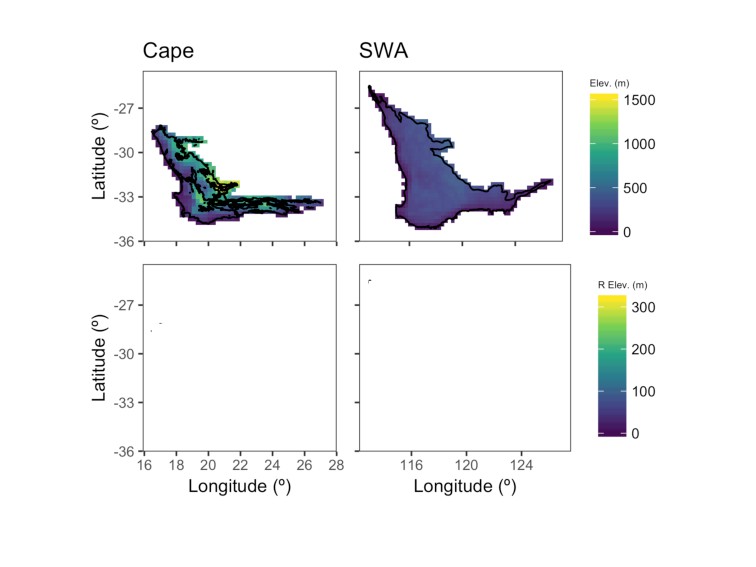
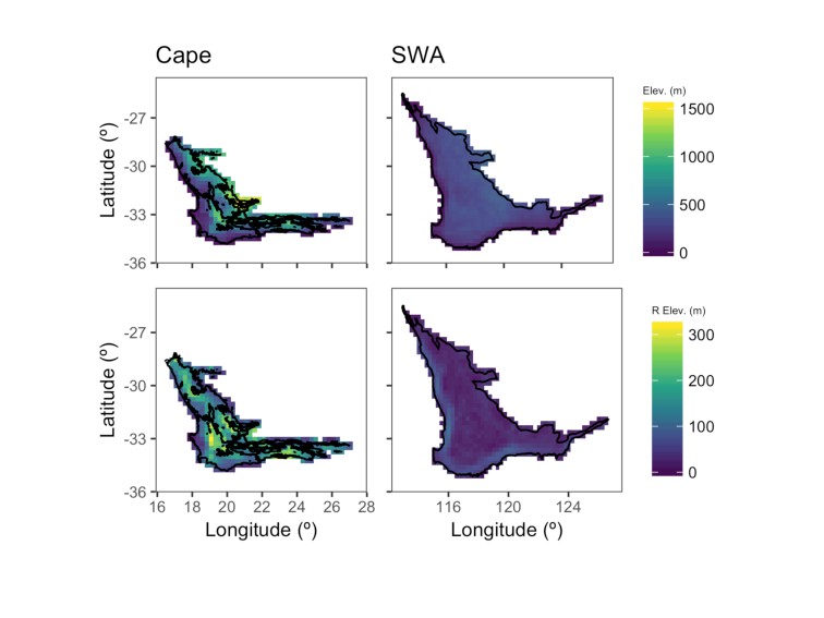
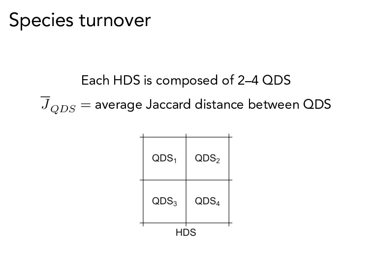
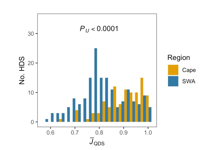
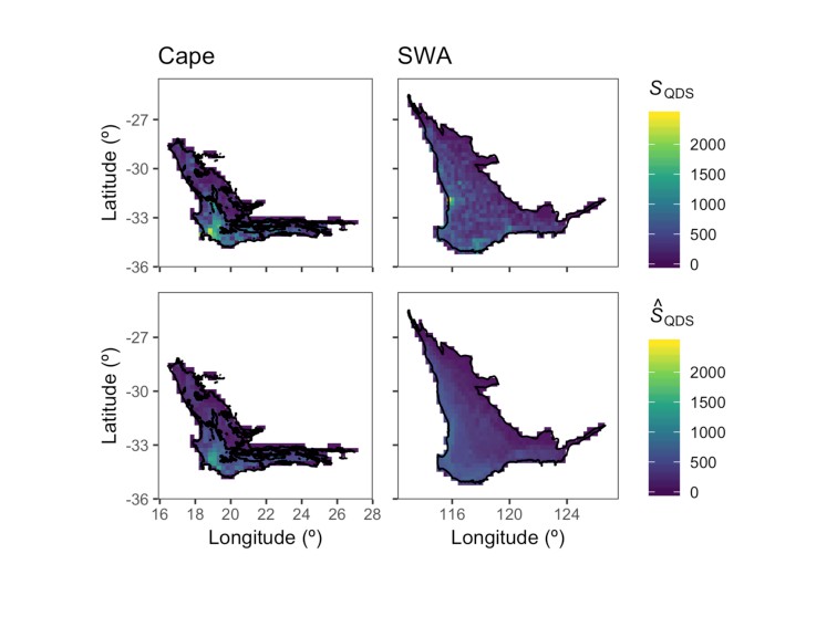
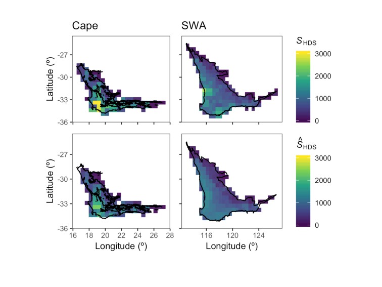
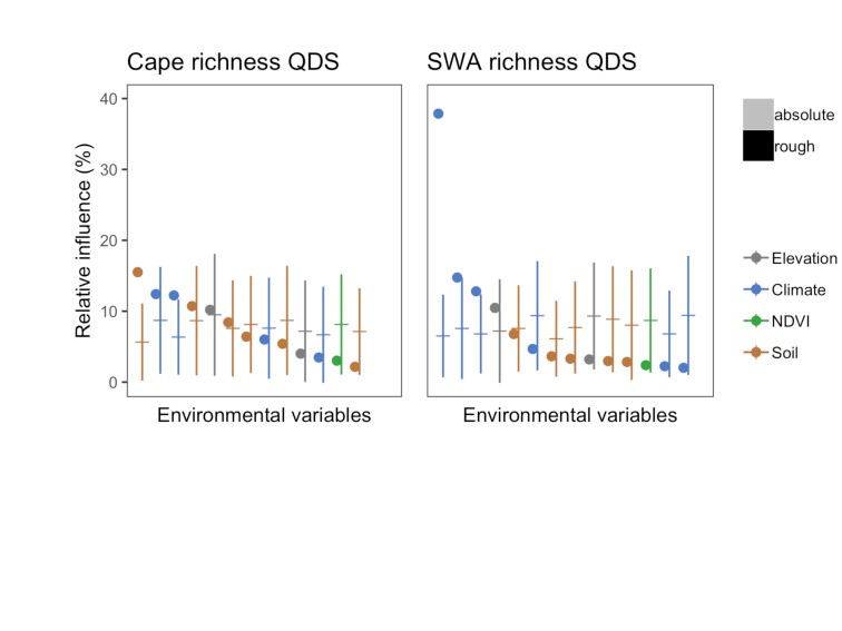
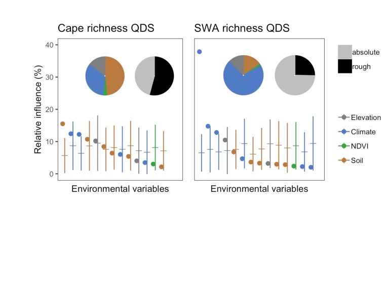
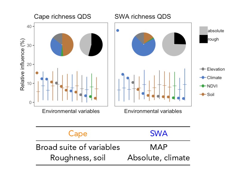
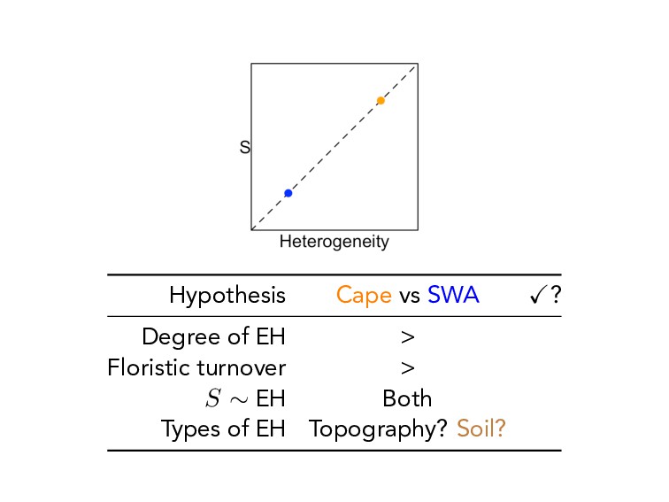
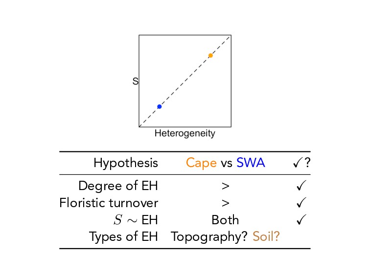
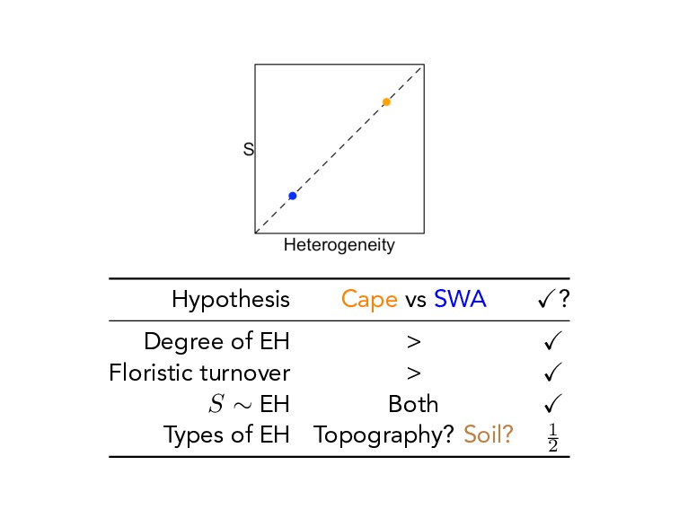
I presented the core findings of work started during my Honours year, comparing macro-ecological models and environmental correlates of species richness in the Cape and SW Australia, at the 45th Joint SAAB-AMA-SASSB Congress. I'd like to acknowledge and thank all the funding received for this project (logos on the coverslide) and the University of Cape Town High Performance Computing Unit for the use of their facilities for the modelling work. Please see the abstract for this oral presentation here. This presentation was created using "rmarkdown", an open source R-package for document preparation, using the beamer presentation output option.

Transcript

1. Environmental turnover predicts plant species richness & turnover Comparing the Greater Cape Floristic Region & the Southwest Australia Floristic Region Silvermine, Table Mountain National Park, South Africa, 2017 © Ruan van Mazijk, Jonathan A. Drake Supervised by Prof M.D. Cramer & A/Prof G.A. Verboom @rvanmazijk Ruan van Mazijk
2. Species richness (Ԉ)
3. Species richness (Ԉ) Speciation Co-existence
4. Species richness (Ԉ) Extremely high Ԉ? Speciation Co-existence
5. Species richness (Ԉ) Environmental heterogeneity (EH) Speciation Co-existence
6. Species richness (Ԉ) Environmental heterogeneity (EH) Speciation along ecological gradients Co-existence within ecological space
7. The Cape & SWA
8. Similar – Environments mediterranean, winter rainfall – Plant ecologies serotiny, sclerophylly
9. But different – Ԉ per unit area Cape > SWA – Topographies mountainous vs flat
10. – EH shown previously as NB in the Cape1 – Does this extend to SWA? 1Cramer & Verboom 2016. J. Biogeography 44(3)
12. Hypothesis Cape vs SWA
13. Hypothesis Cape vs SWA Degree of EH > Floristic turnover >
14. Hypothesis Cape vs SWA Degree of EH > Floristic turnover > Ԉ ୽ EH
15. Hypothesis Cape vs SWA Degree of EH > Floristic turnover > Ԉ ୽ EH Both
16. Hypothesis Cape vs SWA Degree of EH > Floristic turnover > Ԉ ୽ EH Both Types of EH
17. Hypothesis Cape vs SWA Degree of EH > Floristic turnover > Ԉ ୽ EH Both Types of EH Topography? Soil?
18. Data sources – Each region’s boundaries – Environmental data – NASA MODIS, CHIRPS, SoilsGrid250m – Vascular plant occurrence records – GBIF
19. Quantifying EH Local neighbourhood ԃ about cell ԧ ց֊վռև Roughness ԇ ԃ  Ԉӹ ց֊վռև ԃ
23. Species turnover Each HDS is composed of 2–4 QDS ӿ ղեմ  average Jaccard distance between QDS
26. Relating Ԉ & EH: BRT-modelling – Machine-learning – Non-linear, complex & multivariate datasets
27. Relating Ԉ & EH: BRT-modelling – Machine-learning – Non-linear, complex & multivariate datasets ^ S = w 1 + w 2 + w 3 + ... + w n
35. Cape SWA Broad suite of variables MAP Roughness, soil Absolute, climate
37. Hypothesis Cape vs SWA ௡? Degree of EH > Floristic turnover > Ԉ ୽ EH Both Types of EH Topography? Soil?
38. Hypothesis Cape vs SWA ௡? Degree of EH > ௡ Floristic turnover > ௡ Ԉ ୽ EH Both ௡ Types of EH Topography? Soil?
39. Hypothesis Cape vs SWA ௡? Degree of EH > ௡ Floristic turnover > ௡ Ԉ ୽ EH Both ௡ Types of EH Topography? Soil? φ ϵ
40. Conclusions – The Cape is more environmentally heterogeneous than SWA
41. Conclusions – The Cape is more environmentally heterogeneous than SWA – Consequently more species rich – Greater floristic turnover supports this.
42. Conclusions – The Cape is more environmentally heterogeneous than SWA – Consequently more species rich – Greater floristic turnover supports this. – Different axes of EH are biologically important in the Cape and SWA.
43. Conclusions – The Cape is more environmentally heterogeneous than SWA – Consequently more species rich – Greater floristic turnover supports this. – Different axes of EH are biologically important in the Cape and SWA. Soil?
44. Thank you1! 1And an extra thank you to my supervisors, Mike & Tony