Upgrade to Pro — share decks privately, control downloads, hide ads and more …

An introduction to R Markdown

An introduction to R Markdown

A tutorial in literate programming and plain-text document prep using RMarkdown, for my colleagues in the West Lab at the Department of Biological Sciences, University of Cape Town. This presentation was made using RMarkdown with the beamer presentation output option. See the GitHub repository for the source material.
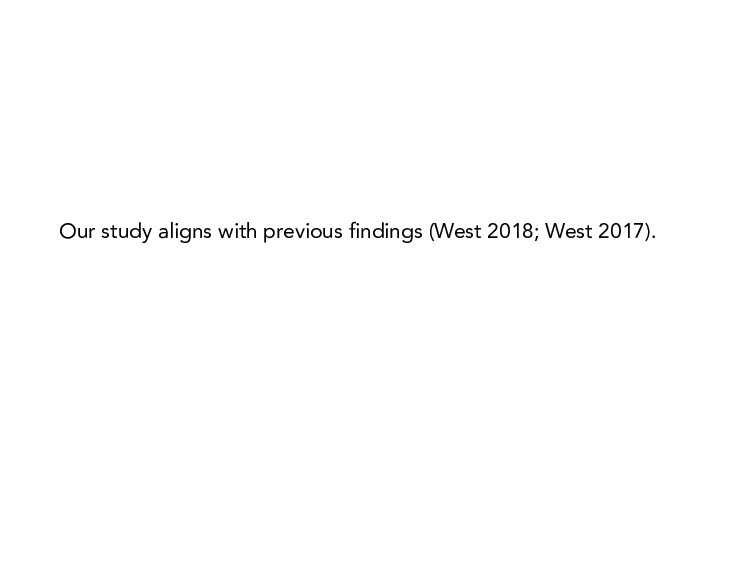
Ruan van Mazijk

January 24, 2019
Tweet

More Decks by Ruan van Mazijk

Other Decks in Programming

Transcript

  1. What is R Markdown? R Markdown is a document preparation

    system, like MS Word, but completely different. Importantly, it works in plain-text and is highly accessible, open source, and makes it really easy to embed R-code in documents (e.g. to create figures or tables).
  2. Document preparation systems Document prep systems vary. There are those

    where what you see is what you get in the final document (“WYSIWYG”-systems; e.g. MS Word), and there are those where what you see is what you mean (“WYSIWYM”-systems; e.g. markup languages such as HTML, LaTeX). R Markdown is based on the markup language “Markdown”. Markdown was invented to be a simpler alternative to more complicated markup languages like HTML and LaTeX. These markup languafes are often quite hard to read in raw-form and even harder to write. See for yourself:
  3. The benefits of R Markdown What R Markdown does is

    extend Markdown by making R-code (and other programming languages) executable from within the document’s source file, allowing the results to show up in the final document (e.g. figures or tables), thereby “weav[ing] together narrative text and code to produce elegantly formatted output” (https://rmarkdown.rstudio.com). It also adds a bit more functionality to Markdown with simple syntax for in-text references, equations, and more. And, best of all, it makes the results of any analysis fully reproducible!
  4. How does R Markdown work? R Markdown takes the file

    you write (e.g. analysis.Rmd), converts it to plain markdown using the R-package knitr, then converts it any of the output formats you choose, using the open source software pandoc. Figure 3: R Markdown flowchart (https://rmarkdown.rstudio.com/lesson-2.html)
  5. Example analysis.Rmd might look like this: --- title: My analysis

    author: Ruan van Mazijk date: 2019-11-15 output: html_document --- # Introduction Blah blah blah blah ... # Methods Etc. etc. etc. ...
  6. Rendering your document Use the output specified in the header

    rmarkdown::render("analysis.Rmd") Or over-ride it rmarkdown::render("analysis.Rmd" output_format = "pdf_document" )
  7. Unordered lists - Item - Item - Item - Sub-item

    - Sub-item - Sub-sub-item - Etc.
  8. Unordered lists cont. ▶ Item ▶ Item ▶ Item ▶

    Sub-item ▶ Sub-item ▶ Sub-sub-item ▶ Etc.
  9. Ordered lists 1. Item 2. Item 3. Item a. Sub-item

    b. Sub-item 1. Sub-sub-item 2. Etc.
  10. Ordered lists cont. 1. Item 2. Item 3. Item a.

    Sub-item b. Sub-item 1..b.1 Sub-sub-item 2..b.2 Etc.
  11. Citations You need a .bib file, which looks like this

    (e.g. example.bib): @article{West2018, author = {West, A.G. et al.}, year = {2018}, title = {A previous study}, journal = {Nature}, number = {50}, volume = {49}, pages = {340--346} } @article{West2017, ... } (Mendeley and other reference managing software can easily generate this file for you from your library.)
  12. And link it to analysis.Rmd in the YAML header: ---

    ... bibliography: example.bib ---
  13. By adding the following heading to the end of analysis.Rmd:

    # References It will automatically produce the reference list!
  14. R-code We can embed figures in our document. echo=FALSE tells

    R Markdown not to display the code chunk that generates the figure. \ ```{r, echo=FALSE} \ plot(cars) \ ``` (Ignore the backslashes)
  15. R-code cont. 5 10 15 20 25 0 20 40

    60 80 100 120 speed dist
  16. Alternatively, we can set echo=TRUE: \ ```{r, echo=TRUE} \ x

    <- 1:100 \ y <- 3 * jitter(x, 100) \ m <- lm(y ~ x) \ visreg::visreg(m) \ ```
  17. x <- 1:100 y <- 3 * jitter(x, 100) m

    <- lm(y ~ x) visreg::visreg(m) 0 20 40 60 80 100 0 100 200 300 x y
  18. Further reading R Markdown “Getting Started” Tutorial. https://rmarkdown.rstudio.com/lesson-1.html. R Mardown

    Cheatsheet. https://rmarkdown.rstudio.com/lesson-15.html. R Markdown Reference Guide. https://www.rstudio.com/wp- content/uploads/2015/03/rmarkdown-reference.pdf. Yihui, X., Allaire, J.J., Grolemund, G. (2018). R Markdown: The Definitive Guide. https://bookdown.org/yihui/rmarkdown/.
  19. References West, A.G. et al. 2017. “An Even Older Study.”

    Nature 32 (46): 189–203. ———. 2018. “A Previous Study.” Nature 49 (50): 340–46.