Programming Complexity

Modeling Complex Systems with Go and React

Transcript

1. Programming   Complexity Modeling  Complex  Systems  with  Go  and  React Chang  Sau Sheong sausheong@gmail.com
2. Complexity The  behavior  that  emerges  from  a  group  of  interacting   parts,  that  is  not  directly  the  result  of  interactions   between  individual  parts
5. Modeling  cultural  interactions
8. The  Dissemination  of  Culture American  political  scientist,  complexity  theory  researcher,   National  Medal  of  Science  laureate Robert  Axelrod
9. Cultures  who  are  similar  to  each  other  are   likely  to  interact
10. When  cultures  interact,  they  become  more   alike  each  other
11. Agent-­‐based  model  where  each  agent   represents  a  culture  
12. Culture  =  Set  of  Features language,  religion,  style  of  dress  etc
13. Trait  =  possible  values  of  a  feature
14. 36  x  36  grid each  cell  has  a  culture culture
15. 5 4 3 2 1 0 Each  culture  has  6  features
16. Each  feature  has  16  possible  traits 0 1 2 3 4 5 6 7 8 9 A B C D E F
19. 8  neighbours
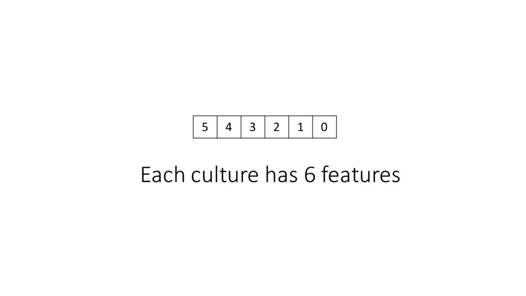
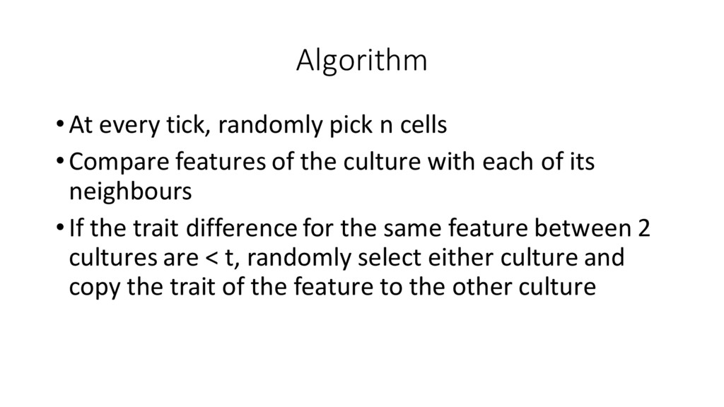
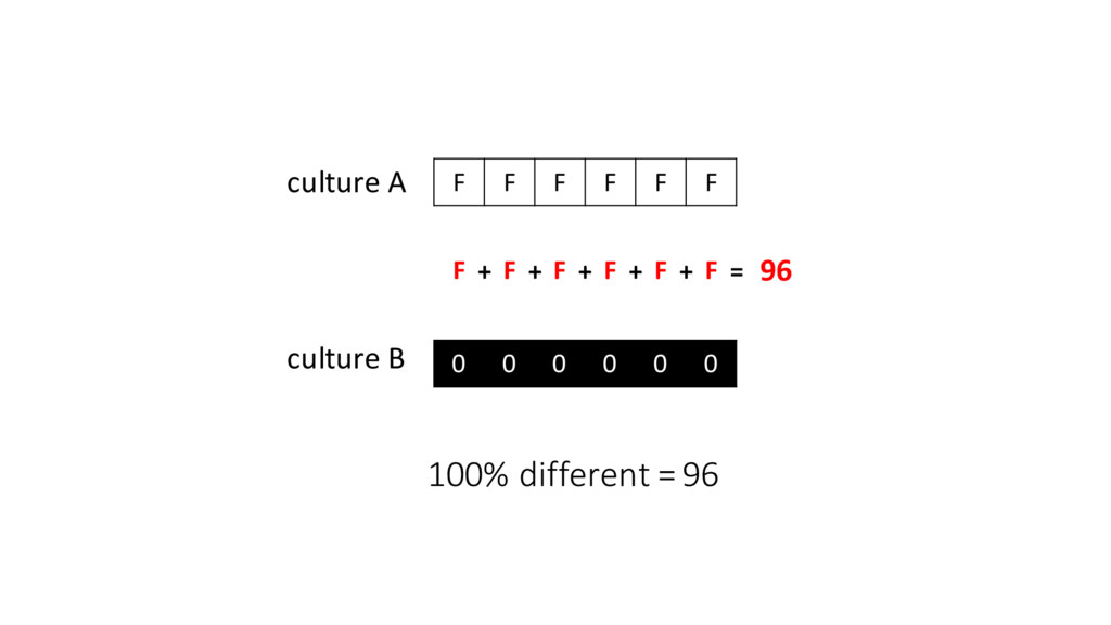
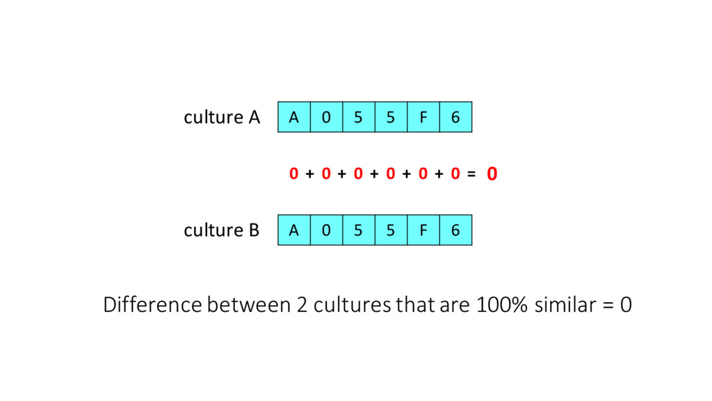
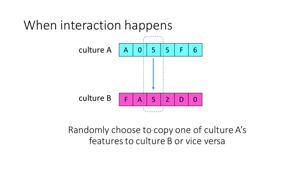
20. Algorithm •At  every  tick,  randomly  pick  n  cells •Compare  features  of  the  culture  with  each  of  its   neighbours •If  the  trait  difference  for  the  same  feature  between  2   cultures  are  <  t,  randomly  select  either  culture  and   copy  the  trait  of  the  feature  to  the  other  culture
21. A B A  and  B  are  2   neighbouring cultures
22. difference  is  5  – 2  =  3 culture  B culture  A A 0 5 5 F 6 F A D 2 D 0
23. A 0 5 5 F 6 F A D 2 D 0 culture  B culture  A Difference  between  2  cultures  =  34 5 A 8 3 2 6 + + + + + = 34
24. F F F F F F 0 0 0 0 0 0 culture  B culture  A 100%  different  =  96 F F F F F F + + + + + = 96
25. A 0 5 5 F 6 culture  B culture  A Difference  between  2  cultures  that  are  100%  similar  =  0 0 0 0 0 0 0 + + + + + = 0 A 0 5 5 F 6
26. The  more  similar  2  cultures  are,  the  more  likely   there  will  be  cultural  exchange Probability  of  cultural  exchange  =  1  -­‐ difference   between  2  cultures  ÷ 96
27. Probability  of  cultural  exchange: 1   −   34 96 = 1   − 0.354 = 64.6%  
28. culture  B culture  A Randomly  choose  to  copy  one  of  culture  A’s   features  to  culture  B  or  vice  versa A 0 5 5 F 6 F A 5 2 D 0 When  interaction  happens
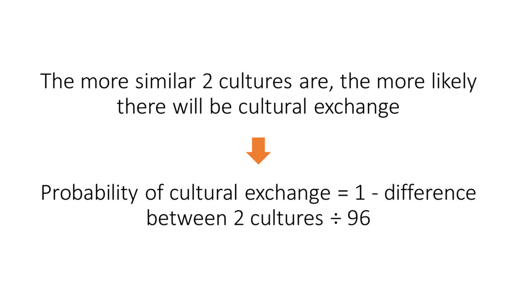
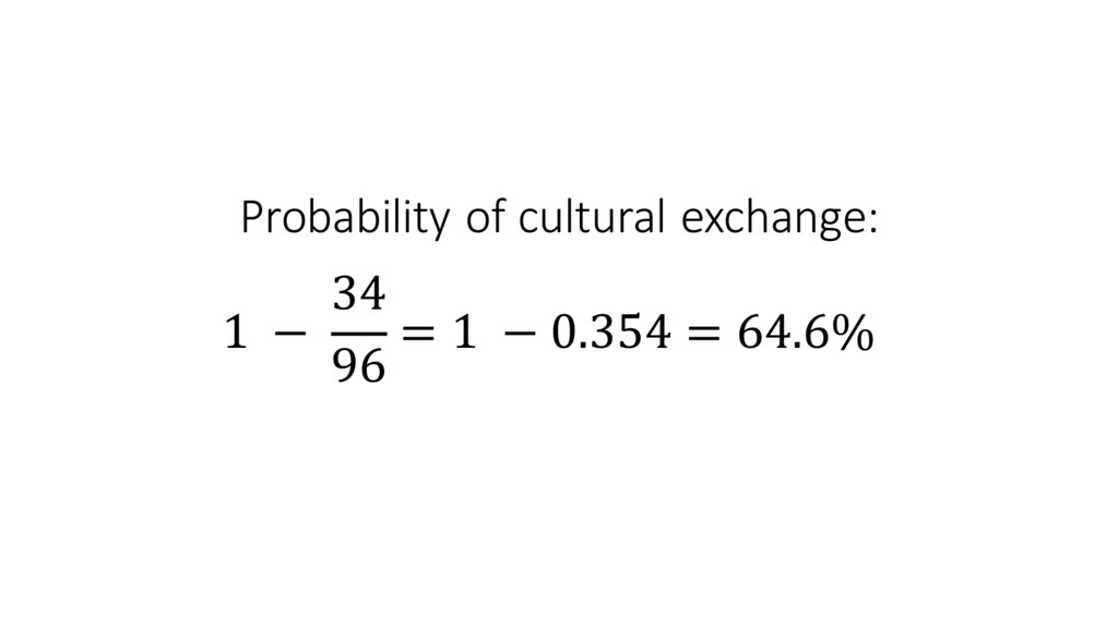
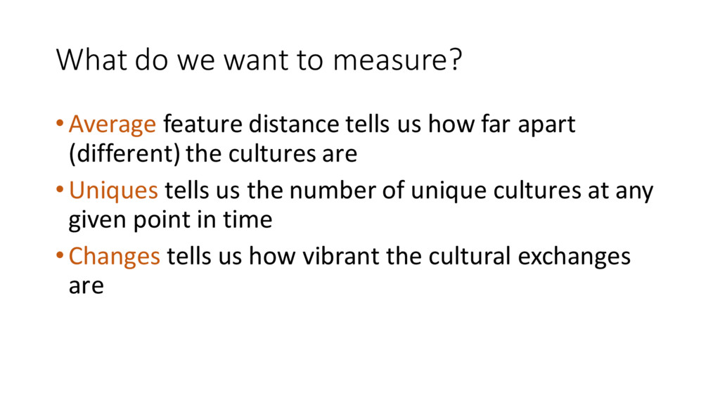
29. What  do  we  want  to  measure? •Average feature  distance  tells  us  how  far  apart   (different)  the  cultures  are •Uniques tells  us  the  number  of  unique  cultures  at  any   given  point  in  time •Changes tells  us  how  vibrant  the  cultural  exchanges   are
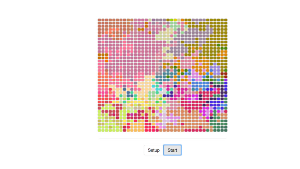
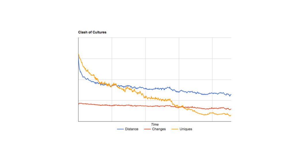
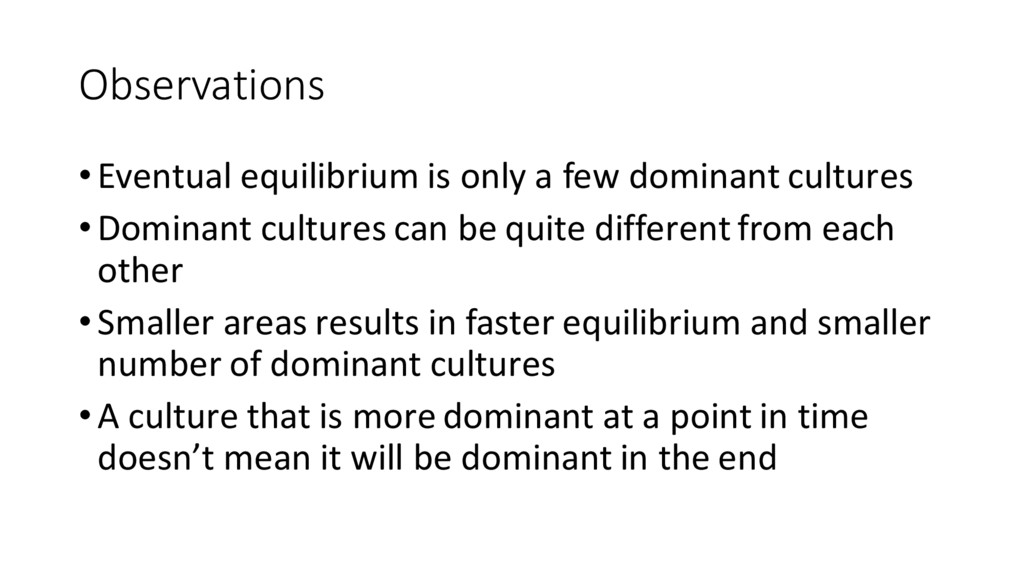
32. Observations •Eventual  equilibrium  is  only  a  few  dominant  cultures •Dominant  cultures  can  be  quite  different  from  each   other •Smaller  areas  results  in  faster  equilibrium  and  smaller   number  of  dominant  cultures •A  culture  that  is  more  dominant  at  a  point  in  time   doesn’t  mean  it  will  be  dominant  in  the  end
33. Modeling  racial   segregation
34. Chicago
35. Washington  D.C. New  York  City Detroit Los  Angeles
36. London
37. Dynamic  Models  of  Segregation American  economist,  2005  Nobel  Prize  in  Economics Thomas  Schelling
38. 36  x  36  grid each  cell  has  a  household
39. 8  neighbours
40. Algorithm •At  every  tick,  check  every  cell •If  at  least  n  number  of  its  neighbours are  of  the  same   ‘race’,  do  nothing •Otherwise,  randomly  pick  an  empty  cell  and  move   there
41. Parameters •Acceptable number  of  neighbours (n) •Number of  ‘races’  in  the  grid  (r) •Percentage  of  vacant  cells  (v) •Policy  limitation – cannot  have  more  than  (l)  number   of  neighbours of  the  same  race
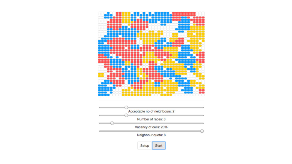
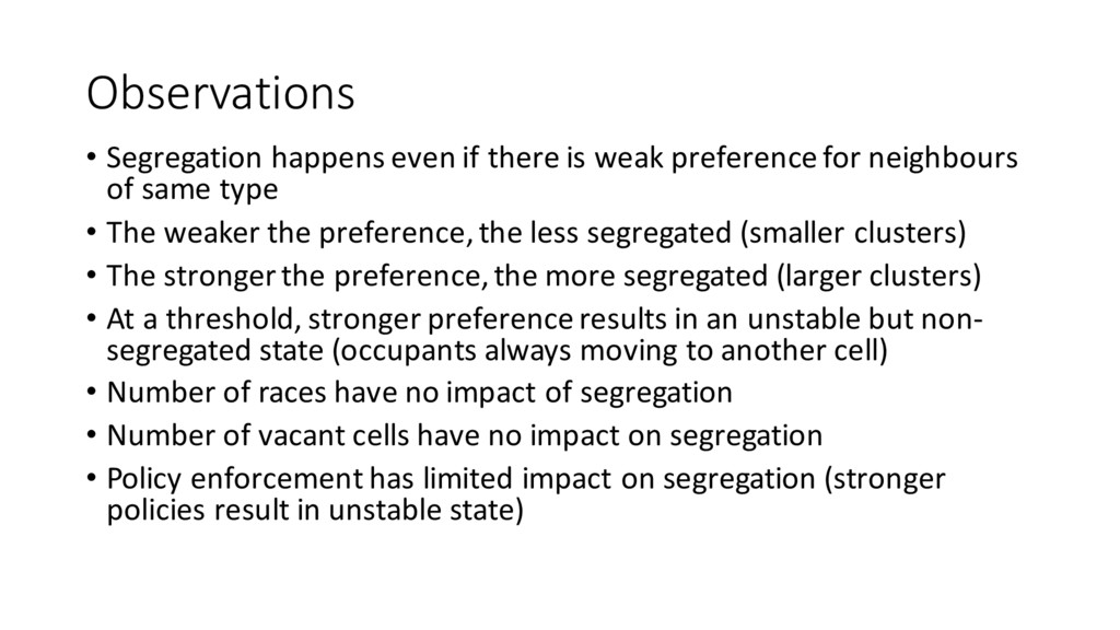
44. Observations • Segregation  happens  even  if  there  is  weak  preference  for  neighbours of  same  type • The  weaker  the  preference,  the  less  segregated  (smaller  clusters) • The  stronger  the  preference,  the  more  segregated  (larger  clusters) • At  a  threshold,  stronger  preference  results  in  an  unstable  but  non-­‐ segregated  state  (occupants  always  moving  to  another  cell) • Number  of  races  have  no  impact  of  segregation • Number  of  vacant  cells  have  no  impact  on  segregation • Policy  enforcement  has  limited  impact  on  segregation  (stronger   policies  result  in  unstable  state)
45. Modeling  bystander  effect
49. Game  Theory
50. The  study  of  mathematical  models  of  conflict  and   cooperation,  often  used  in  economics  and  political   science
51. Volunteer’s  Dilemma
52. V  =  value  gained  if  at  least  1  person  volunteers C  =  individual  cost  of  volunteering A =  overall  cost  if  no  one  volunteers
53. You volunteer You  don’t   volunteer I volunteer I  don’t  volunteer V  -­ C V  -­ C V  -­ C V V  -­ C V V  -­ A V  -­ A Payoff  matrix  for  a  2-­‐player  game
54. You  volunteer You don’t   volunteer I volunteer I  don’t  volunteer V  -­ C V  -­ C V  -­ C V V  -­ C V V  -­ A V  -­ A If  I  volunteer
55. You  volunteer You  don’t   volunteer I volunteer I  don’t  volunteer V  -­ C V  -­ C V  -­ C V V  -­ C V V  -­ A V  -­ A If  I  don’t volunteer
56. Mixed  strategy  Nash  equilibrium V  – C  =  pV +  (1  – p)(V  – A)   where  p  =  probability  of  volunteering  
57. For  an  N-­‐player  game Probability  of  volunteering  =  p  x  p  x  …  x  p =  pN-­‐1 N  – 1  times
58. For  an  N-­‐player  game Probability  of  not  volunteering  =  (1  – p)N-­‐1
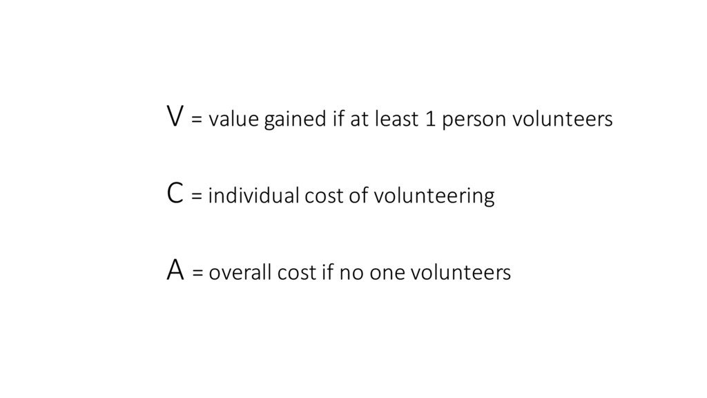
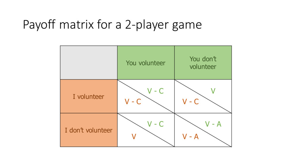
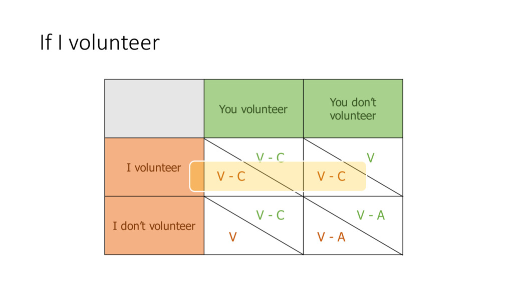
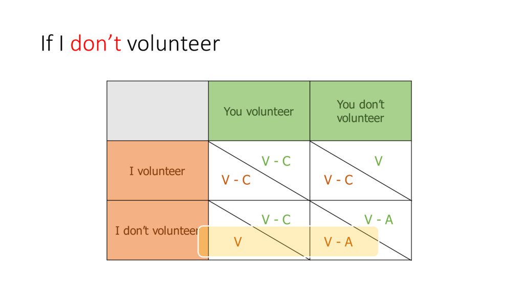
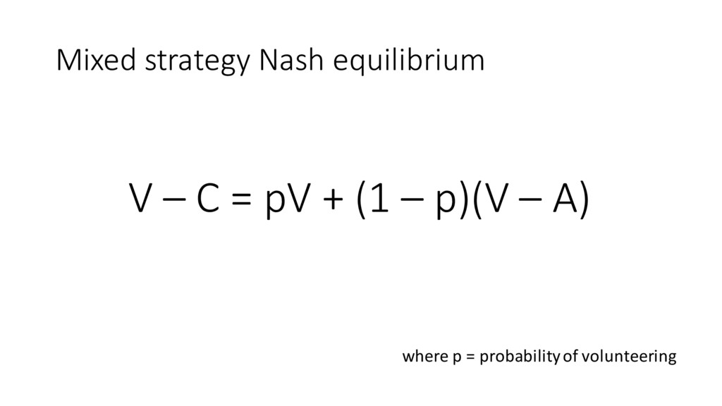
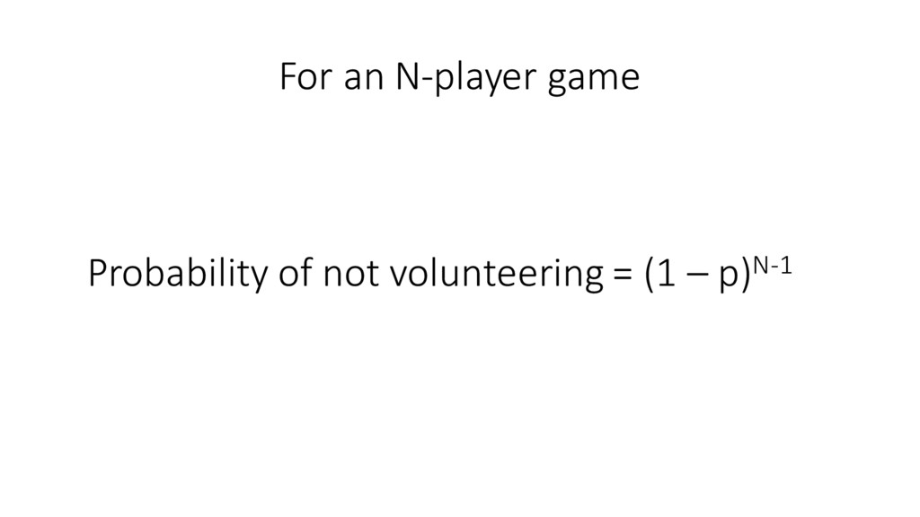
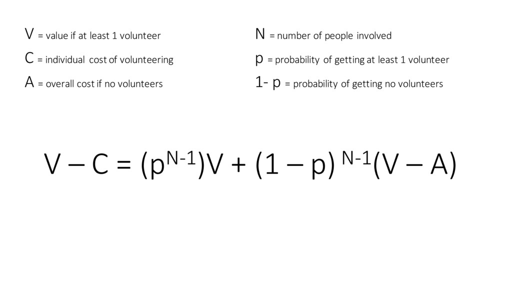
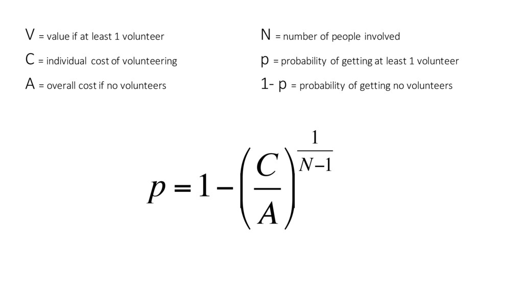
59. V  =  value  if  at  least  1  volunteer C  =  individual   cost  of  volunteering A  =  overall  cost  if  no  volunteers N  =  number  of  people  involved p  =  probability  of  getting  at  least  1  volunteer 1-­‐ p  =  probability  of  getting  no  volunteers V  – C  =  (pN-­‐1)V  +  (1  – p) N-­‐1(V  – A)  
60. V  =  value  if  at  least  1  volunteer C  =  individual   cost  of  volunteering A  =  overall  cost  if  no  volunteers N  =  number  of  people  involved p  =  probability  of  getting  at  least  1  volunteer 1-­‐ p  =  probability  of  getting  no  volunteers p =1− C A " # $ % & ' 1 N−1
61. Monte  Carlo  simulation
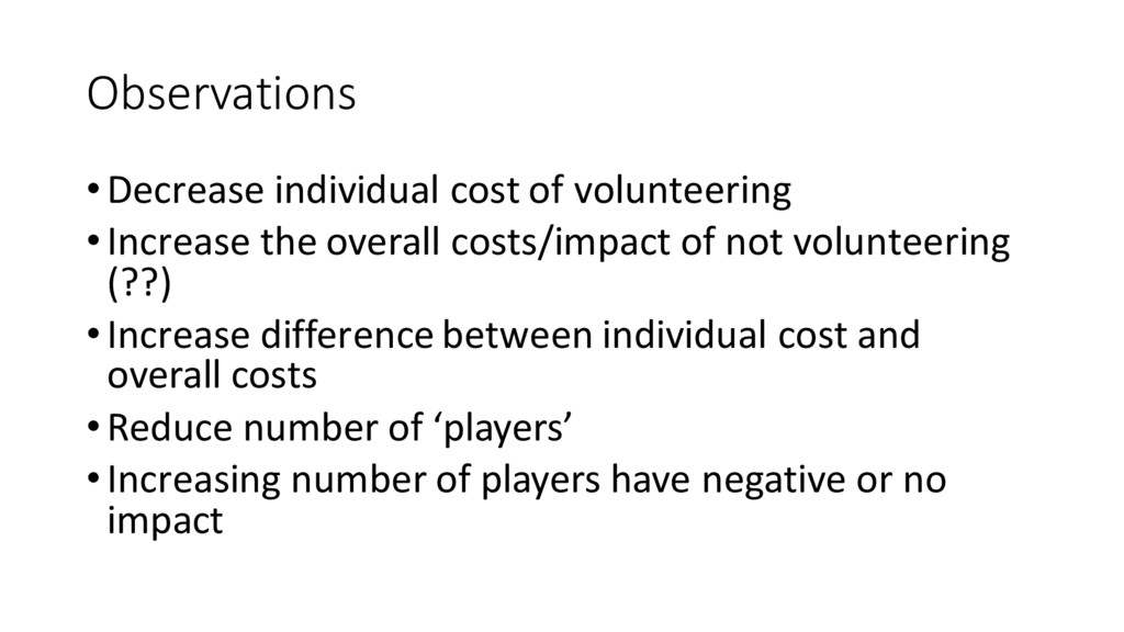
64. Observations •Decrease  individual  cost  of  volunteering •Increase  the  overall  costs/impact  of  not  volunteering   (??) •Increase  difference  between  individual  cost  and   overall  costs •Reduce  number  of  ‘players’ •Increasing  number  of  players  have  negative  or  no   impact
65. @sausheong sausheong@gmail.com http://blog.saush.com http://github.com/sausheong