Kolmogorov complexity & applications. Time series anomaly discovery with grammar-based compression.

Transcript

1. Kolmogorov complexity & applications Time series anomaly discovery with grammar-based compression Pavel Senin senin@hawaii.edu 1
2. Understanding the information • We live in a society driven by information, undeniably: • But do we know, what “information” is mathematically? • How to quantify it? Or to assess its quality? • How to use it for research, or to prove a theorem? • How to refine it? 2
3. Information quantification, beginning • Turned out these questions were asked long before the information become ubiquitous. • As Lance Fortnow noted, 1903 was an interesting year: first flight was made and three men were born. The three who happened to be quite determined in finding the answers: – Alonzo Church (adviser of Alan Turing) – John von Neumann – Andrey Kolmogorov First flight, Orville and Wilbur Wright 3
4. Key work introducing Kolmogorov complexity • “Three approaches to the quantitative definition of information”, A.N. Kolmogorov, 1965. • Discusses approaches: – Combinatorial, Ralph Hartley, 1928 • Probability-independent (sampled uniformly at random) • Can be seen as a Shannon entropy for uniform distribution • Non negative value – Probabilistic, Claude E. Shannon, 1948 • Probabilistic assumptions • May produce a negative value (differential entropy) • Proposes: – Algorithmic, based on the “true information content”. 4
5. Solomonoff – Kolmogorov – Chaitin Solomonoff (1960)-Kolmogorov (1965)-Chaitin (1969) The amount of information in a string is the size of the smallest program of an optimal Universal TM generating that string 5
6. • Assume there are n mutually exclusive alternatives, and one of them is true, but we don’t know which (equiprobable). • How we can measure the amount of information gained by knowing which one is true, or equivalently, the uncertainty that is associated with these n possibilities? • Hartley postulated that this function, SH ,shall satisfy a set of axioms while mapping natural numbers to real: – Monotonicity SH (n)≤ SH (n+1) – Branching (additivity) SH (nm) = SH (n) + SH (m) – Normalization SH (2) = 1 • Naturally, there is exactly one function satisfying these, which is logarithm, i.e. SH (n) = log n. Hartley function (1927) (Ralph Hartley, Lake Como Italy, “Transmission of information”) 6
7. • Shannon entropy properties hold only when a characteristic probabilities (distributions) of the source are known. • Message is a random sample or characters drawn from a data stream. Shannon entropy is the expected value of the information contained in each message received. • Entropy characterizes the uncertainty about the source of information, and increases for more sources of greater randomness. max is when all events are equiprobable. • The less likely the message is, the more information it provides when it is received. Shannon entropy (1948) (later generalized by Alfréd Rényi, 1961) 7
8. • Kolmogorov proposed to change the paradigm. Kolmogorov (i.e. algorithmic) complexity  “Discrete forms of storing and processing information are fundamental…”  “…it is not clear why information theory should be based so essentially on the probability theory …”  “…the foundations of information theory must have a finite combinatorial character.” • In contrast to previous measures, Kolmogorov’s approach deals with finite sequences, i.e. obtained from a source with unknown characteristics. 8
9. Kolmogorov’s heat conductivity example         ∂ ∂ + ∂ ∂ + ∂ ∂ = ∂ ∂ 2 2 2 2 2 2 z u y u x u t u α General, exact form of the heat equation representing the continuous process of the heat transfer: ) ( u u u u zz yy xx t ∆ + ∆ + ∆ = ∆ α practical, universally used difference scheme: “…Quite probably, with the development of novel computing technique it will be clear that in very many cases it is reasonable to conduct the study of real phenomena avoiding the intermediately stage of stylizing them in the spirit of ideas of mathematics of the infinite and the continuous, and passing directly to discrete models…” A.N. Kolmogorov, 1970, Nice, France, International Congress of Mathematicians 9
10. Computability (applicability boundaries) 1. Partial recursive function, and the lambda-calculus are well-grounded theories which provide a formal system in mathematical logic for expressing a process of computation. 2. Church hypothesis (Church-Turing thesis): The class of algorithmically computable functions (i.e. with paper and ink) coincides with the class of all partial recursive functions. We assume a Turing machine equivalence to lambda calculus. 3. In addition to that, there exist definitions of a universal Turing machine which can simulate any arbitrary Turing machine on an arbitrary input. We assume the existence of a universal Turing machine, a universal partial recursive function, and their equivalence. • Resume: the computers are as powerful as humans, and the Universe is equivalent to a Turing machine, or maybe Universe is a hypercomputer capable of computing super-recursive functions… 10
11. Kolmogorov complexity (conditional) • Say we are interested in finding out the quantity of information object Y conveys about object X. • The computability theory gives us a formalism that if X and Y can be expressed as numbers, there exists a computable (partial recursive) function Φ (P, Y) = X, where P is the “program” describing the computation constructively. • Then, the Kolmogorov complexity is the size of the smallest such program. – as there are many possible programs, “…it is natural to consider only minimal in length numbers P that lead to the object …”. 11
12. For strings X and Y, an interpreter A, and the program p (just assume that A is a Turing machine) Kolmogorov formulated and proved the fundamental theorem in his work, that there exists a partial recursive function U, that for any other partial recursive function A Kolmogorov complexity The proof of this asymptotically optimal function existence is based on the existence of universal partial recursive function. 12
13. – this is an equivalent of undecidability of the Halting problem – this is also a reflection of Kurt Gödel incompleteness theorem (a system capable of expressing elementary arithmetic cannot be both consistent and complete. i.e. for a system that proves certain arithmetic truths, there exists a an arithmetical statement that is true, but not provable in the system) • Getting around: by using a compressor, i.e. gzip. Or JPEG. The better it compresses the string x, the better it approximates K(x). (lossy JPEG is questionable… but it works). The catch “… it is important to note, that partial recursive functions are not defined everywhere, and there is no fixed method for determining whether application of the program P to an object k will lead to result or not…” 13
14. Summary on K-complexity • The Kolmogorov complexity deals with the complexity of objects and defines it as the size of the shortest binary program capable of the object’s generation – a fascinating concept describing an object’s complexity by scientific means. • The concept of “the shortest program” was developed by Solomonoff, Kolmogorov, and Chaitin independently while working on Turing machines, random objects, and inductive inference. Whereas Solomonoff worked on the idealized inference and universal prior and Chaitin worked on Turing machinery properties, Kolmogorov proposed the complexity measure directly. • The field of Kolmogorov complexity, while mature, is still active research area where many research problems still to be solved. 14
15. Some properties and implications • For all x, K(x) ≤ |x|+O(1) (upper bound) • K(xx) = K(x) + O(1) (a loop over a program) • K(x|x) = O(1) (just print out input) • K(x|ε) = K(x) (empty set provides no information) • K(x|y) < K(x) +O(1) (at worst y has no value) • K(1n ) ≤ K(logn) (the sequence’ encoding length) • K(π1:n ) ≤ K(logn)(there is a short program generating π ) • C(xy) ≤ C(x) + C(y) + O(log(min{C(x),C(y)}) (additivity) 15
16. Applications (I). Randomness. A case of cheating casino* • Bob proposes to flip a coin with Alice: – Alice wins a euro if Heads; – Bob wins a euro if Tails… • Result: TTTTTT …. 100 Tails in a roll. – Alice lost € 100. She feels being cheated… * Courtesy of M. Li and P. Vitaniy, Lectures on Kolmogorov Complexity 16
17. Randomness. Alice goes to court* * Courtesy of M. Li and P. Vitaniy, Lectures on Kolmogorov Complexity • Alice complains: T100 is not random. • Bob asks Alice to produce a random coin flip sequence. • Alice flipped her coin 100 times and got THTTHHTHTHHHTTTTH … • But Bob claims Alice’s sequence has probability 2-100, and so does his. • How do we define randomness? 17
18. Randomness • By computing the Kolmogorov complexity, or approximating it, we essentially compress the object. • Incompressibility: for constant c>0, a string x ε {0,1}* is c-incompressible if K(x) ≥ |x|-c. – for a constant c, we simply say that x is incompressible. – i.e., a string is called compressible if it has a description which is shorter than the string itself. • Incompressible strings lack regularities that could be exploited to obtain a compressed description for them; they are effectively patternless. • For a FINITE string x, we say that x is random if K(x) ≥ |x| - c, for a small constant c. 18
19. Randomness, Alice goes to court* • S0 = TTTTT, 100 tails in a row – K(S0) is small, “print ‘T’ 100 times” ~ 20 characters • S1 = THTTHHTHTHHHTTTTH – K(S1) = ???, if truly random, then K(S1)>100 characters • Lemma. There are at least 2n – 2n-c +1 c-incompressible strings of length n. Proof. There are only ∑k=0,…,n-c-1 2k = 2n-c -1 programs with length less than n-c. Hence only that many strings (out of total 2n strings of length n) can have shorter programs (descriptions) than n-c. QED. * Courtesy of M. Li and P. Vitaniy, Lectures on Kolmogorov Complexity 19
20. Randomness • P. Martin-Lof visited Kolmogorov in Moscow 1964-1965 • We may have zillions of statistical tests for randomness. – A random sequence must have roughly ½ 0’s and ½ 1’s, furthermore, ¼ 00’s, 01’s, 10’s 11’s. – A random sequence of length n cannot have a large block of 0’s. – ….. • A truly random sequence shall pass all such tests! • A set of all possible tests should be enumerable. Martin-Lof defined a universal P-test for randomness using that fact. And, he has shown that if a sequence passes the universal test, it passes all enumerated tests. • Then Martin Lof has shown that an effective randomness test cannot distinguish incompressible strings from “truly random” strings if their length exceeds a constant (depending on the test)… I.e., all incompressible strings whose length is greater than this constant pass the universal test. 20
21. Summary on randomness • Kolmogorov complexity effectively enables the definition of incompressible (i.e. random strings). K(x) ≥ |x|-c. • There is a lot of incompressible strings. – 2n – 2n-c +1 of c-incompressible strings of length n. • Per Martin-Löf provided a theoretical framework which proves that incompressible sequences are in fact random. 21
22. Applications (II). Incompressibility method. • A general-purpose method for formal proofs which can be used as an alternative to counting arguments or probabilistic arguments. • To show that in average case the objects in a given class have a certain property: 1. Choose a random object from the class. 2. This object is incompressible, with probability 1. 3. Prove that the property holds for the object. 4. Assume that the property does not hold. 5. Show that we can use the property to compress the object, yielding a contradiction. 22
23. Incompressibility example. Theorem: there are infinitely many primes.* • Suppose not, and there are k primes (p1 ,..,pk ). • Then, any m is a product of these: • Let m be a Kolmogorov-random number of length n • m can be described as above by k numbers (ei ). • ei <log(m), => |ei |<log(log(m)), => |(ei ,…,ek )| < 2k log(log(m)) • as m<2n+1, |(ei ,…,ek )|<2k log(n+1), and K(m)<2k log(n+1)+C. • but, for a large m, K(m)>n, since m is random! • Contradiction, so there are infinitely many primes. * The example from lectures by Lance Fortnow, prepared from notes of the author taken by Amy Gale in Kaikoura, January 2000. 23
24. A selected list of results proven with the incompressibility method (summary)* • Ω(n2) for simulating 2 tapes by 1 (20 years) • k heads > k-1 heads for PDAs (15 years) • k one-ways heads can’t do string matching (13 yrs) • 2 heads are better than 2 tapes (10 years) • Average case analysis for heapsort (30 years) • k tapes are better than k-1 tapes. (20 years) • Many theorems in combinatorics, formal language/automata, parallel computing, VLSI • Simplify old proofs (Hastad Lemma). • Shellsort average case lower bound (40 years) * Courtesy of M. Li and P. Vitaniy, Lectures on Kolmogorov Complexity 24
25. Applications (III). Minimum description length. • MDL is a formalization of Occam’s razor. – among competing hypotheses that predict equally well, the one with the fewest assumptions should be selected – given set of data, the best description is the one that leads to the best compression of the data (i.e. shortest description) • Introduced in 1978, Jorma Rissanen. • MDL “…is based on the following insight: any regularity in a given set of data can be used to compress the data, i.e. to describe it using fewer symbols than needed to describe the data literally..." (Grünwald, 1998). 25
26. MDL in patterns mining. • Pattern mining is an important concept in data mining contrasting to modeling. Patterns describe only the data. – Think motif sequence discovery (i.e. domains, repeats) in bioinformatics • Obviously, there are way too many possible patterns to examine each candidate. • Typically this issue handled with minimum support threshold. But that is only a part of solution, because support threshold does not limit redundancy. • MDL helps here – we use patterns that compress the dataset most. 26
27. Patterns mining. The KRIMP algorithm. http://www.patternsthatmatter.org/ Vreeken, J., Van Leeuwen, M., & Siebes, A. (2011). Krimp: mining itemsets that compress. Data Mining and Knowledge Discovery, 23(1), 169-214. 27
28. • Patterns in data can be ranked by their ability to compress the dataset. • Equally sound models can be ranked by their complexity/assumptions. • This technique (philosophy) is general and can be applied across research areas and applications. • Use carefully, if none of the distributions under consideration represents the data generating machinery very well, MDL fails. https://xkcd.com/1155/ MDL, summary 28
29. Applications (IV). Information Distance. (This is my favorite) • Enables measuring the distance between digital objects: – Two genomes (evolution) – Two documents (plagiarism detection, authorship/subject recognition) – Two computer programs (virus detection) – Two emails (signature verification) – Two pictures – Two homepages – Two songs – Two youtube movies * Image example - courtesy of M. Li and P. Vitaniy, Lectures on Kolmogorov Complexity 29
30. Normalized Information Distance Normalized Compression Distance (using bzip, gzip, winrar) Normalized Google Distance (pages containing x, y, and x and y together) 30
31. Whole Genome Phylogeny Li et al, Bioinformatics, 2001 • Uses all the information in the genome; no need of evolutionary model – universal; no need of multiple alignment • Eutherian Orders problem: it has been a disputed issue which of the two groups of placental mammals are closer: Ferungulates, Primates, or Rodents? In mtDNA: - 6 proteins say primates closer to ferungulates; - 6 proteins say primates closer to rodents 31
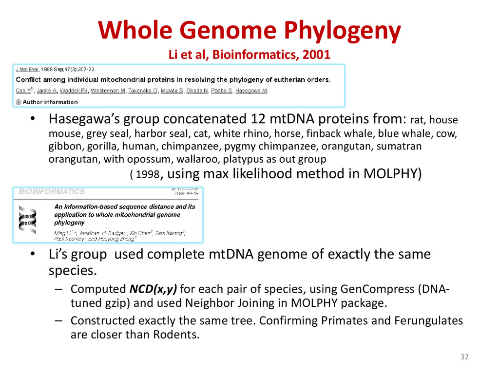
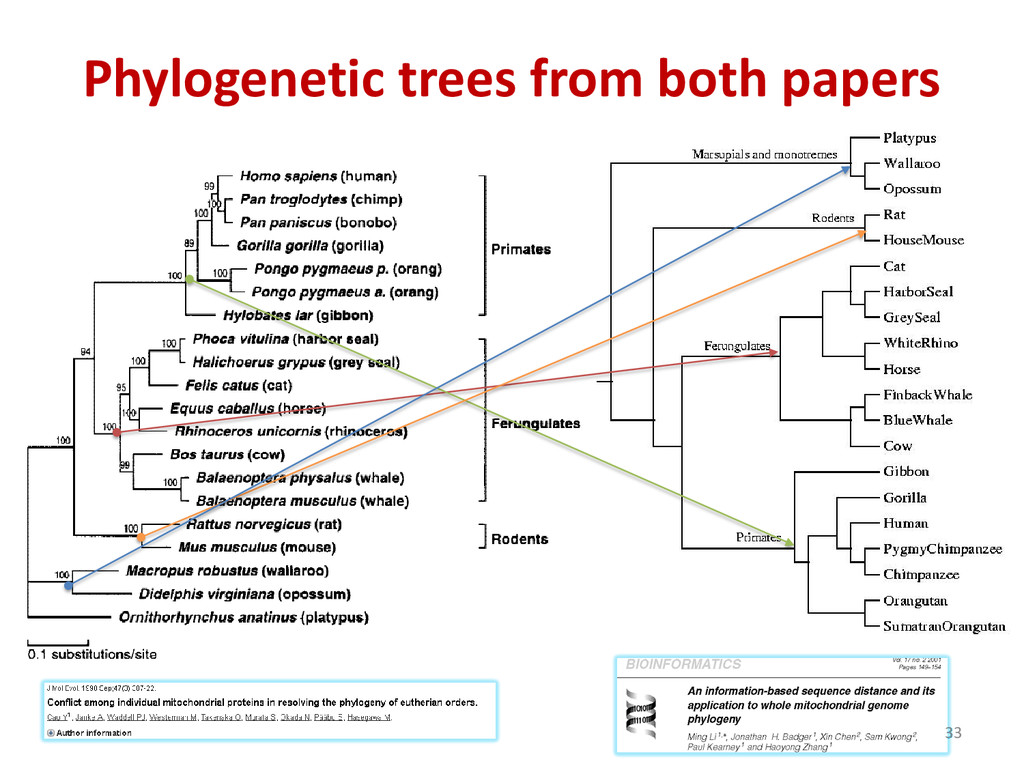
32. Whole Genome Phylogeny Li et al, Bioinformatics, 2001 • Hasegawa’s group concatenated 12 mtDNA proteins from: rat, house mouse, grey seal, harbor seal, cat, white rhino, horse, finback whale, blue whale, cow, gibbon, gorilla, human, chimpanzee, pygmy chimpanzee, orangutan, sumatran orangutan, with opossum, wallaroo, platypus as out group ( 1998, using max likelihood method in MOLPHY) • Li’s group used complete mtDNA genome of exactly the same species. – Computed NCD(x,y) for each pair of species, using GenCompress (DNA- tuned gzip) and used Neighbor Joining in MOLPHY package. – Constructed exactly the same tree. Confirming Primates and Ferungulates are closer than Rodents. 32
33. Phylogenetic trees from both papers 33
34. Summary on information distance • Normalized compression distance is way of measuring the similarity between two objects. • General, i.e. not application-dependent. It is a truly "parameter-free, feature-free" data-mining tool. • Can be used for clustering of heterogeneous data. • Use Google search engine as a compressor useful for data mining. 34
35. Applications (V). Time series anomaly. Planetary orbits, 10/11th century ICU display Shape to time series transform Trajectory to time series transform 35
36. Classic approaches • Brute force all-with-all comparison • Simple statistics – Compute distribution – Make a decision base on likelihood • Complex statistics – HMM • Transformation into a feature space, such as DFT, DWT, etc. • Current state of the art: HOT-SAX discord discovery algorithm 36
37. Our approach. • In our approach we follow steps suggested by Kolmogorov exactly: 1. Continuous signal discretization (SAX) via sliding window • reduces the dimensionality greatly • enables variable length pattern discovery 2. Grammatical compression (Sequitur) • effective and efficient technique dynamically compresses the discretized signal into a set of rules • enables variable length pattern discovery 3. Conditional Kolmogorov complexity K(X|Y) • at any time our algorithm is able to pinpoint anomalies with respect to the observed signal 37
38. Performance evaluation (orders of magnitude faster than current state of the art) 38 • We propose two algorithms for variable-length anomaly discovery: 1. Rule density curve for approximate anomaly discovery • rule coverage counting, linear time and space, online anomaly discovery 2. Rare Rule Anomaly (RRA) for exact anomaly discovery • HOTSAX modification, heuristics uses ranked grammatical rules (after GI, |terminals|+|non_terminals| ≤ |terminals|, thus less calls to distance function)
39. Step 1: Symbolic Aggregate Approximation 0 - - 0 20 40 60 80 100 120 b b b a c c c a 0 20 40 60 80 100 120 C C baabccbc 39 We pass a sliding window along the time series extracting a sequence of words
40. Step 2: Discretized time series to context-free grammar with Sequitur Input: abcabcabcXXXabcabc Output: 40
41. R2 R2 R2 Step 3: Grammar structure analysis, rule density curve Input: abcabcabc XXX abcabc Output: R2 R2 R1 Coverage depth 2 Coverage depth 1 Coverage depth = 0, i.e. incompressible Anomaly! Coverage depth 2 41 R1
42. Live demonstration https://www.youtube.com/watch?v=9lH-RG5OtkY 42
43. How good Sequitur is? (better than gzip, worse than arithmetic coding) Table by Richard Ladner, U. Washington. 43
44. Applications. Trajectory data. • The trajectory data is intrinsically complex to explore for regularity since patterns of movement are often driven by unperceived goals and constrained by unknown environmental settings. • The data used in this study was gathered from a GPS device which recorded location coordinates and times while commuting during a typical week on foot, by car, and bicycle. • To apply RRA to the trajectory, the multi-dimensional trajectory data (time, latitude, longitude) was transformed into a sequence of scalars. 44
45. Hilbert space-filling curve (1891) • The trajectory becomes a sequence of scalars {0,3,2,2,2,7,7,8,11,13,13,2,1,1}, i.e., a time series! 45
46. Finding an anomaly in Hilbert curve-transformed trajectory Planted anomaly, traveled once A week of typical commute 46
47. Examples of true anomalies discovered in the trajectory data Abnormal behavior of not visiting the parking lot Abnormal path outside from a highly visited area (similar to the planted anomaly) 47
48. Discretization parameters sensitivity analysis 48
49. Resume • Kolmogorov complexity, when approximated with a compressor, enables the ranking of objects based on their information context. • This ranking is general, effective, and efficient. • Conditional Kolmogorov complexity enables information quality assessment. – how much new information was added? – what is the nature of the observed information? • Kolmogorov complexity enables the quantification of algorithmic randomness enabling the discovery of unusual (incompressible) data entities. 49
50. Thank you! • Jessica Lin, Xing Wang, George Mason University, Department of Computer Science. • Tim Oates, Sunil Gandhi, University of Maryland, Baltimore County, Department of Computer Science. • Arnold P. Boedihardjo, Crystal Chen, Susan Frankenstein, U.S. Army Corps of Engineers, Engineer Research and Development Center. • Paul Vitanyi, CWI (for pointers, the book, and lecture slides). 50