R A M E W O R K F O R R O B U S T & R E P R O D U C I B L E B I O M A R K E R D I SC O V E RY F R O M I N T E G R AT E D D ATAS E T S SHEA CONNELL - UNIVERSITY OF EAST ANGLIA
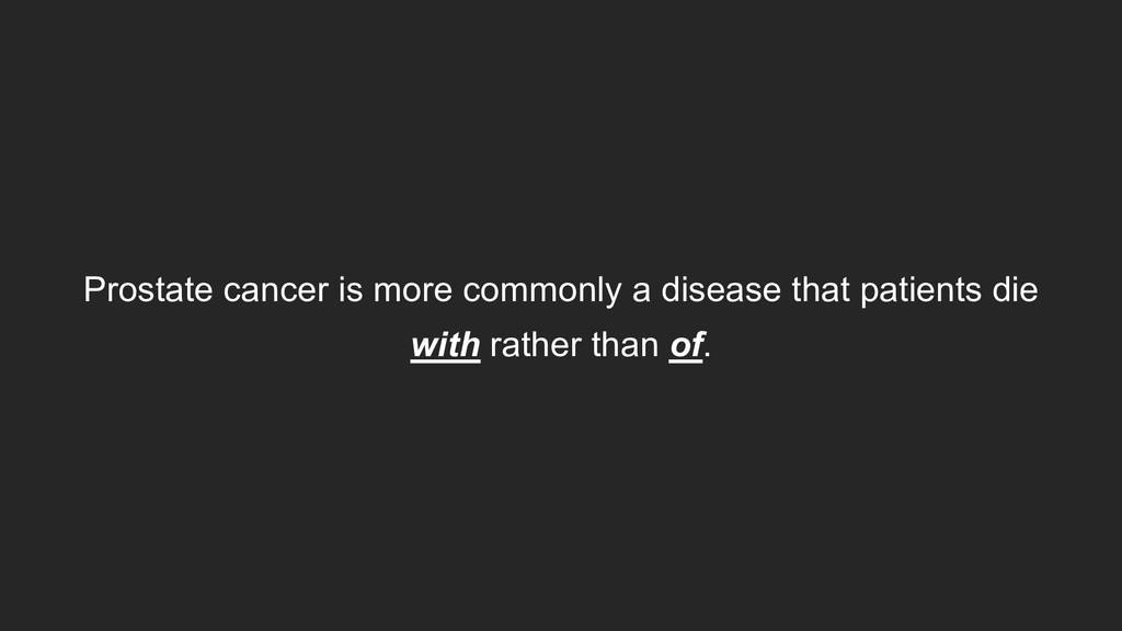
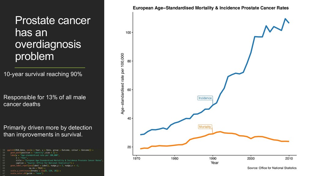
Responsible for 13% of all male cancer deaths Primarily driven more by detection than improvements in survival. Incidence Mortality 20 40 60 80 100 1970 1980 1990 2000 2010 Year Age−standardised rate per 100,000 European Age−Standardised Mortality & Incidence Prostate Cancer Rates Source: Office for National Statistics Prostate cancer has an overdiagnosis problem 10-year survival reaching 90% Responsible for 13% of all male cancer deaths Primarily driven more by detection than improvements in survival. Incidence Mortality 20 40 60 80 100 1970 1980 1990 2000 2010 Year Age−standardised rate per 100,000 European Age−Standardised Mortality & Incidence Prostate Cancer Rates Source: Office for National Statistics
Develop potential diagnostic models robustly, reproducibly & better than standards of care. • Adhere to the TRIPOD guidelines for reporting the development of such a model. • Make the process easy to adapt to new data.
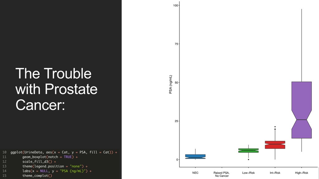
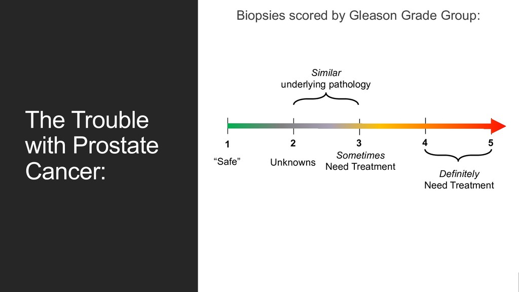
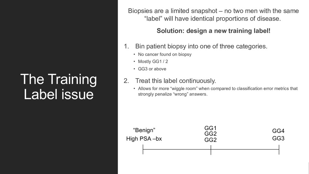
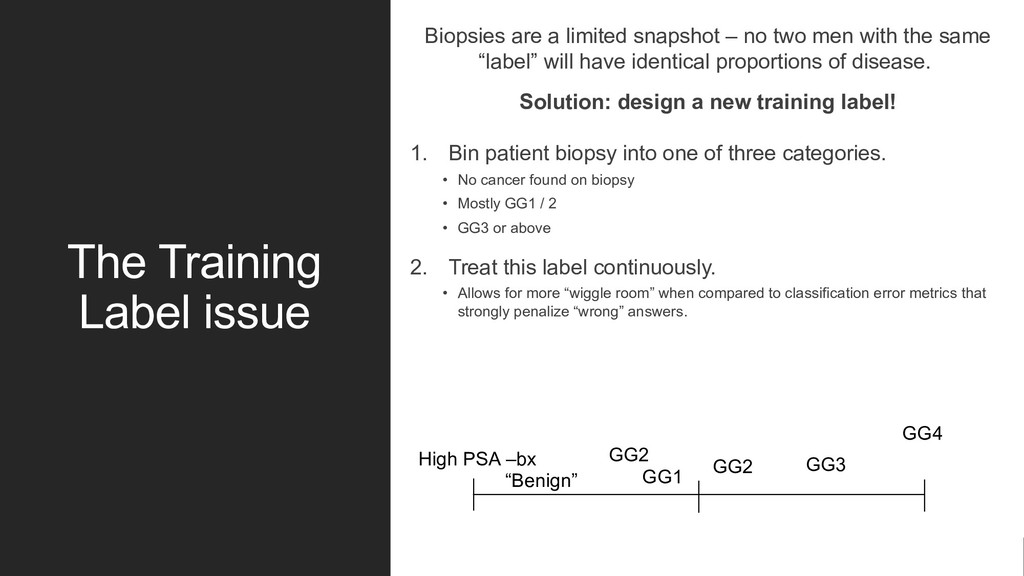
no two men with the same “label” will have identical proportions of disease. Solution: design a new training label! 1. Bin patient biopsy into one of three categories. • No cancer found on biopsy • Mostly GG1 / 2 • GG3 or above 2. Treat this label continuously. • Allows for more “wiggle room” when compared to classification error metrics that strongly penalize “wrong” answers. GG2 GG2 GG1 High PSA –bx GG3 GG4 “Benign”
no two men with the same “label” will have identical proportions of disease. Solution: design a new training label! 1. Bin patient biopsy into one of three categories. • No cancer found on biopsy • Mostly GG1 / 2 • GG3 or above 2. Treat this label continuously. • Allows for more “wiggle room” when compared to classification error metrics that strongly penalize “wrong” answers. GG2 GG2 GG1 High PSA –bx GG3 GG4 “Benign”
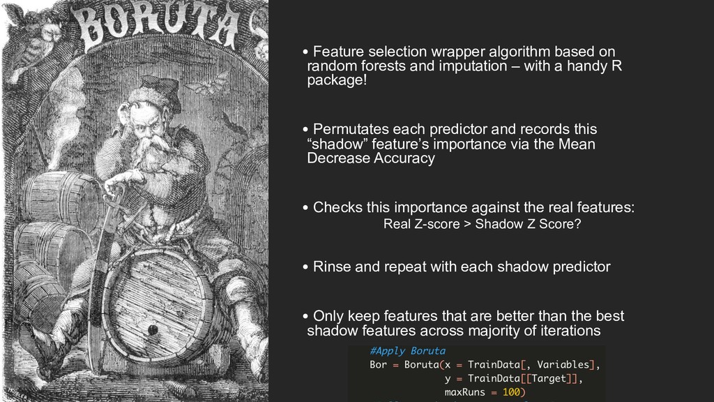
imputation – with a handy R package! • Permutates each predictor and records this “shadow” feature’s importance via the Mean Decrease Accuracy • Checks this importance against the real features: Real Z-score > Shadow Z Score? • Rinse and repeat with each shadow predictor • Only keep features that are better than the best shadow features across majority of iterations
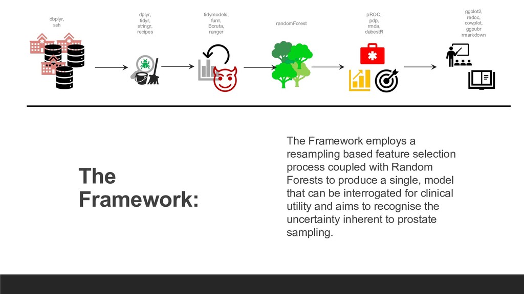
process coupled with Random Forests to produce a single, model that can be interrogated for clinical utility and aims to recognise the uncertainty inherent to prostate sampling. dbplyr, ssh dplyr, tidyr, stringr, recipes tidymodels, furrr, Boruta, ranger randomForest pROC, pdp, rmda, dabestR ggplot2, redoc, cowplot, ggpubr rmarkdown
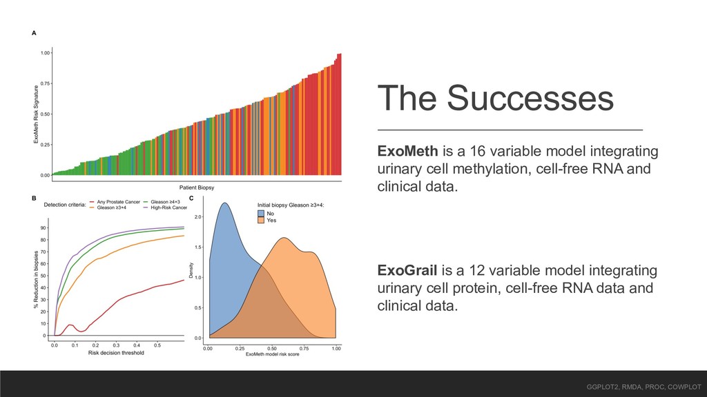
cell methylation, cell-free RNA and clinical data. ExoGrail is a 12 variable model integrating urinary cell protein, cell-free RNA data and clinical data. GGPLOT2, RMDA, PROC, COWPLOT
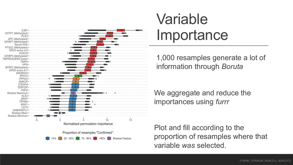
Boruta We aggregate and reduce the importances using furrr Plot and fill according to the proportion of resamples where that variable was selected. FURRR, STRINGR, BORUTA, GGPLOT2
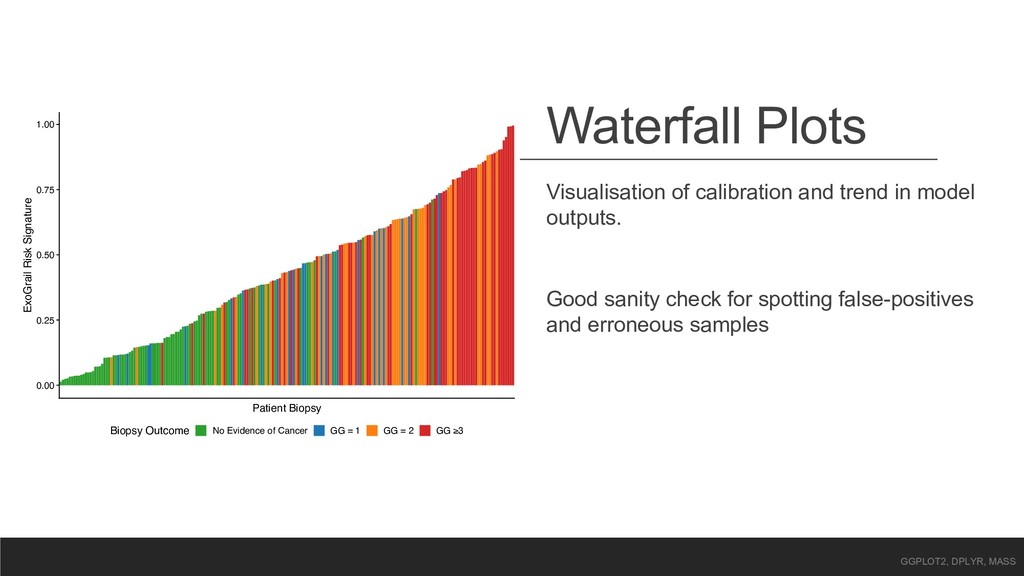
Risk Signature Biopsy Outcome No Evidence of Cancer GG = 1 GG = 2 GG ≥3 Visualisation of calibration and trend in model outputs. Good sanity check for spotting false-positives and erroneous samples GGPLOT2, DPLYR, MASS
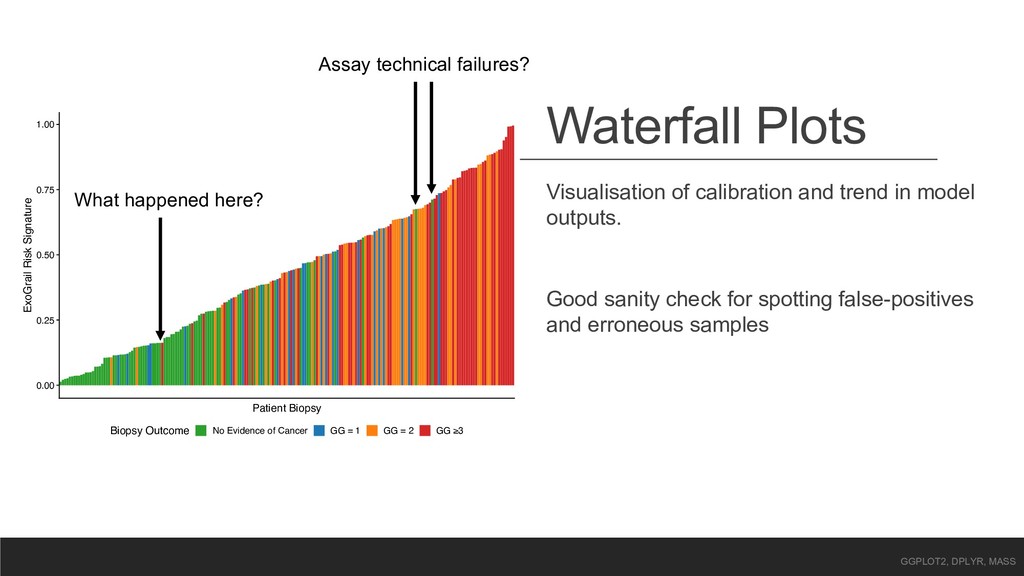
Risk Signature Biopsy Outcome No Evidence of Cancer GG = 1 GG = 2 GG ≥3 Visualisation of calibration and trend in model outputs. Good sanity check for spotting false-positives and erroneous samples GGPLOT2, DPLYR, MASS Assay technical failures? What happened here?
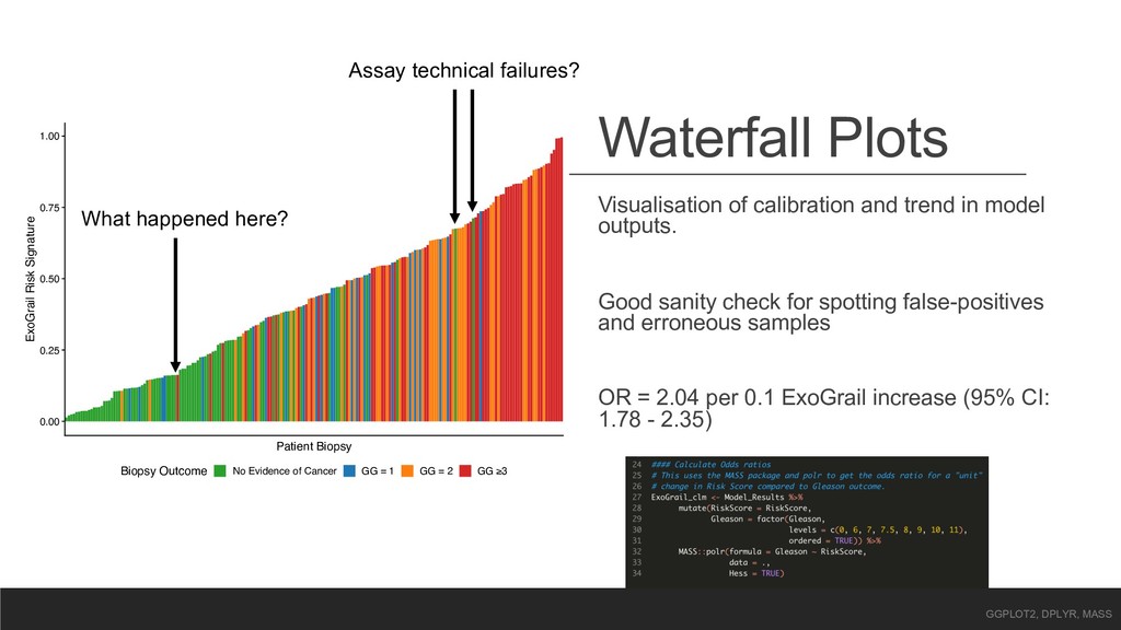
Risk Signature Biopsy Outcome No Evidence of Cancer GG = 1 GG = 2 GG ≥3 Visualisation of calibration and trend in model outputs. Good sanity check for spotting false-positives and erroneous samples OR = 2.04 per 0.1 ExoGrail increase (95% CI: 1.78 - 2.35) GGPLOT2, DPLYR, MASS Assay technical failures? What happened here?
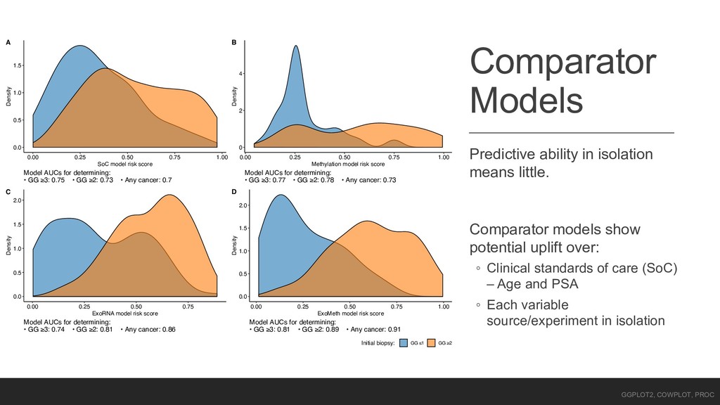
show potential uplift over: ◦ Clinical standards of care (SoC) – Age and PSA ◦ Each variable source/experiment in isolation 0.0 0.5 1.0 1.5 0.00 0.25 0.50 0.75 1.00 SoC model risk score Density Model AUCs for determining: • GG ≥3: 0.75 • GG ≥2: 0.73 • Any cancer: 0.7 A 0 2 4 0.00 0.25 0.50 0.75 1.00 Methylation model risk score Density Model AUCs for determining: • GG ≥3: 0.77 • GG ≥2: 0.78 • Any cancer: 0.73 B 0.0 0.5 1.0 1.5 2.0 0.00 0.25 0.50 0.75 ExoRNA model risk score Density Model AUCs for determining: • GG ≥3: 0.74 • GG ≥2: 0.81 • Any cancer: 0.86 C 0.0 0.5 1.0 1.5 2.0 0.00 0.25 0.50 0.75 1.00 ExoMeth model risk score Density Model AUCs for determining: • GG ≥3: 0.81 • GG ≥2: 0.89 • Any cancer: 0.91 D Initial biopsy: GG ≤1 GG ≥2 GGPLOT2, COWPLOT, PROC
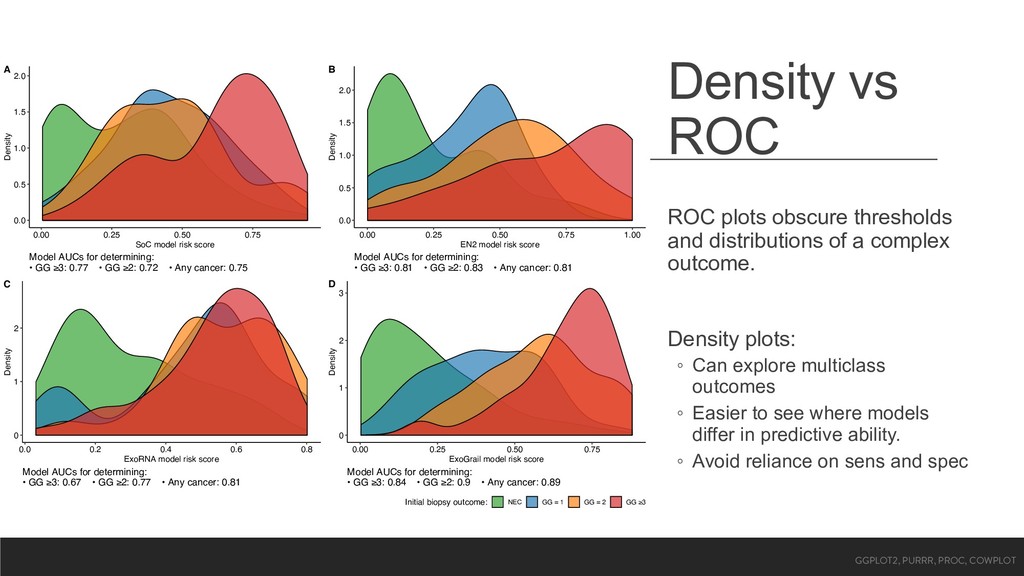
a complex outcome. Density plots: ◦ Can explore multiclass outcomes ◦ Easier to see where models differ in predictive ability. ◦ Avoid reliance on sens and spec 0.0 0.5 1.0 1.5 2.0 0.00 0.25 0.50 0.75 SoC model risk score Density Model AUCs for determining: • GG ≥3: 0.77 • GG ≥2: 0.72 • Any cancer: 0.75 A 0.0 0.5 1.0 1.5 2.0 0.00 0.25 0.50 0.75 1.00 EN2 model risk score Density Model AUCs for determining: • GG ≥3: 0.81 • GG ≥2: 0.83 • Any cancer: 0.81 B 0 1 2 0.0 0.2 0.4 0.6 0.8 ExoRNA model risk score Density Model AUCs for determining: • GG ≥3: 0.67 • GG ≥2: 0.77 • Any cancer: 0.81 C 0 1 2 3 0.00 0.25 0.50 0.75 ExoGrail model risk score Density Model AUCs for determining: • GG ≥3: 0.84 • GG ≥2: 0.9 • Any cancer: 0.89 D Initial biopsy outcome: NEC GG = 1 GG = 2 GG ≥3 GGPLOT2, PURRR, PROC, COWPLOT
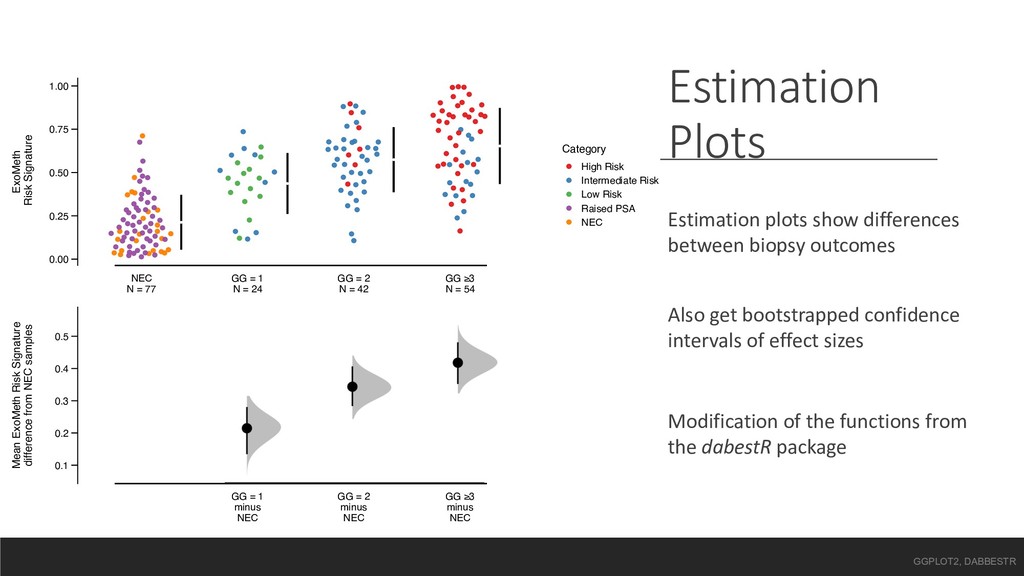
= 1 N = 24 GG = 2 N = 42 GG ≥3 N = 54 ExoMeth Risk Signature Category High Risk Intermediate Risk Low Risk Raised PSA NEC 0.1 0.2 0.3 0.4 0.5 GG = 1 minus NEC GG = 2 minus NEC GG ≥3 minus NEC Mean ExoMeth Risk Signature difference from NEC samples Estimation Plots Estimation plots show differences between biopsy outcomes Also get bootstrapped confidence intervals of effect sizes Modification of the functions from the dabestR package GGPLOT2, DABBESTR
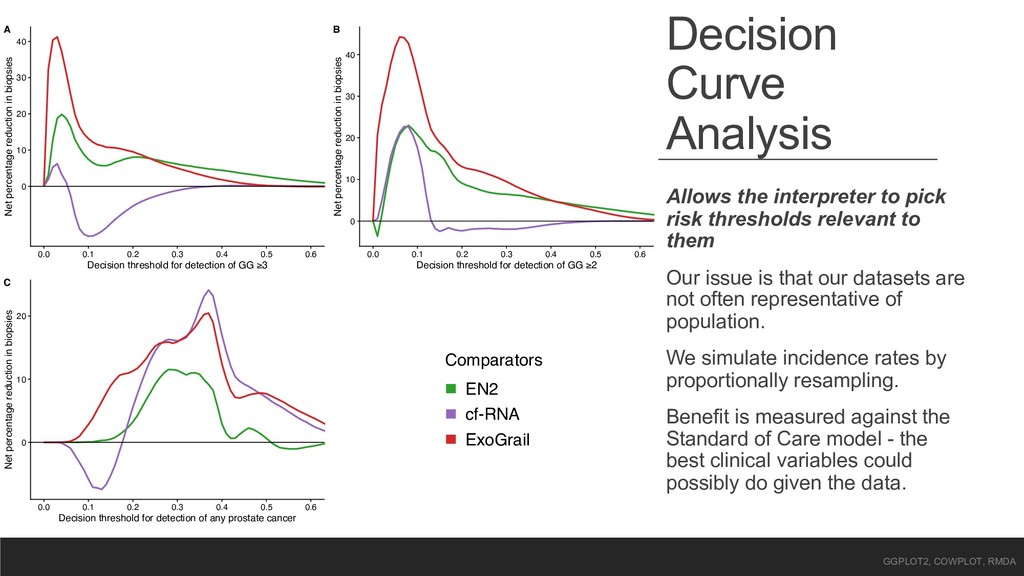
relevant to them Our issue is that our datasets are not often representative of population. We simulate incidence rates by proportionally resampling. Benefit is measured against the Standard of Care model - the best clinical variables could possibly do given the data. 0 10 20 30 40 0.0 0.1 0.2 0.3 0.4 0.5 0.6 Decision threshold for detection of GG ≥3 Net percentage reduction in biopsies A 0 10 20 30 40 0.0 0.1 0.2 0.3 0.4 0.5 0.6 Decision threshold for detection of GG ≥2 Net percentage reduction in biopsies B 0 10 20 0.0 0.1 0.2 0.3 0.4 0.5 0.6 Decision threshold for detection of any prostate cancer Net percentage reduction in biopsies C Comparators EN2 cf-RNA ExoGrail GGPLOT2, COWPLOT, RMDA
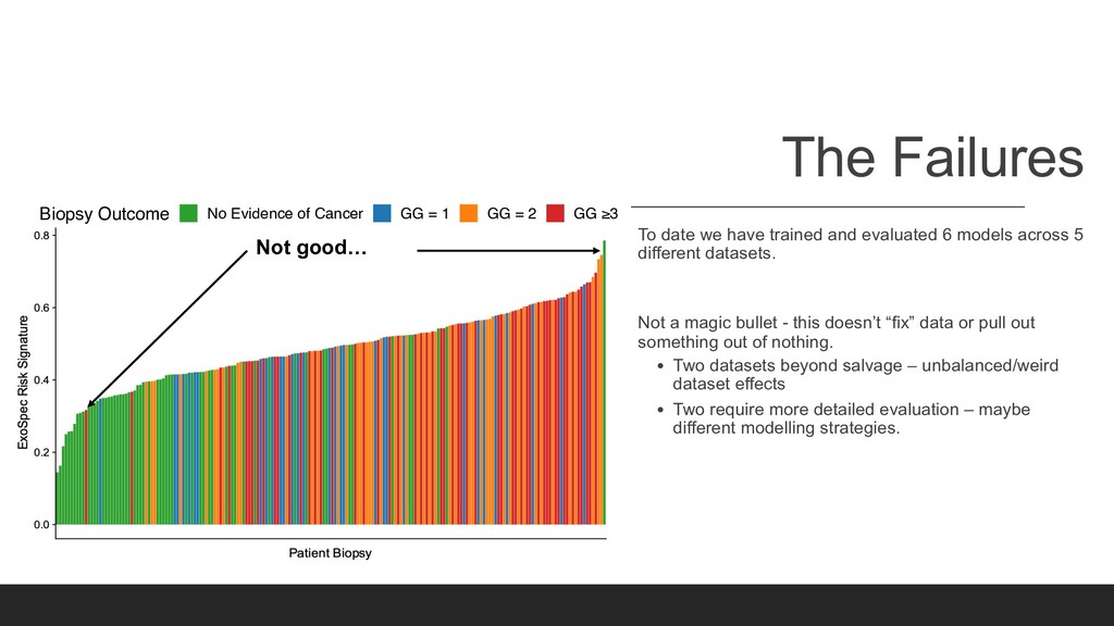
models across 5 different datasets. Not a magic bullet - this doesn’t “fix” data or pull out something out of nothing. • Two datasets beyond salvage – unbalanced/weird dataset effects • Two require more detailed evaluation – maybe different modelling strategies. Not good… Patient Biopsy Biopsy Outcome No Evidence of Cancer GG = 1 GG = 2 GG ≥3
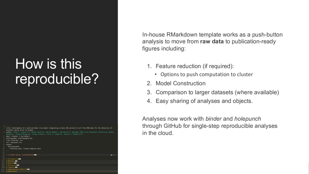
push-button analysis to move from raw data to publication-ready figures including: 1. Feature reduction (if required): • Options to push computation to cluster 2. Model Construction 3. Comparison to larger datasets (where available) 4. Easy sharing of analyses and objects. Analyses now work with binder and holepunch through GitHub for single-step reproducible analyses in the cloud.
have more reasonable lists of targets for new prospective trials and basic research. • Which have been designed around TRIPOD guidelines – to refine these models before true clinical validation. Make plots interactive. Still a handful of datasets to process and investigate – a few months not years. Make all analyses and code openly available to all collaborators and the wider scientific community (uphill battle)