Cloud Computing Lecture (German)

A lecture in german language about cloud computing.

Transcript

1. Cloud Computing Sven Koschnicke
2. Motivation • Es werden immer schneller immer mehr Daten gesammelt • Algorithmen, die auf grossen Datenmengen arbeiten, erfordern viele Resourcen • Umsetzung erforderte hohen finanziellen Aufwand 2
3. 3 Bild von: www.cloudtweaks.com
4. ? 4
5. Definition: National Institute for Standards and Technology (NIST) 5
6. Grundsätzliche Eigenschaften • On-demand self-service • Broad network access • Resource pooling • Rapid elasticity • Measured service 6
7. Deployment Models • Private cloud • Community cloud • Public cloud • Hybrid cloud 7
8. Service Modelle Platform as a Service (PaaS) Infrastructure as a Service (IaaS) Software as a Service (SaaS) 8
9. 9 Bild von: www.cloudtweaks.com
10. Software as a Service • Daten werden zentral gespeichert • Software kann auf mehreren „beliebigen“ Geräten verwendet werden • meist Web-Applikation 10 Platform as a Service (PaaS) Infrastructure as a Service (IaaS) Software as a Service (SaaS)
11. Beispiele 11
12. Platform as a Service • Betrieb von Software in der Cloud • Vorgabe von • Entwicklungsmethoden • Programmiersprachen • Komponenten 12 Platform as a Service (PaaS) Infrastructure as a Service (IaaS) Software as a Service (SaaS)
13. Unterarten • Application PaaS (aPaaS) • Integration and Governance PaaS (iPaaS) • add-on-PaaS 13
14. Beispiele Amazon Elastic Beanstalk Google AppEngine 14
15. Heroku • One-Command deploy and scalability • direkte Unterstützung für Ruby, Node.js, Clojure, Java, Python und Scala > git push heroku > heroku ps:scale web=10 15
16. Infrastructure as a Service • Mieten von • Recheninstanzen (Rechenleistung) • Speicherplatz • beliebige Menge • beliebiger Zeitraum • nur Nutzung wird berechnet 16 Platform as a Service (PaaS) Infrastructure as a Service (IaaS) Software as a Service (SaaS)
17. Beispiele Rackspace Cloud JiffyBox 17 ... Google Compute Engine
18. Amazon Web Services 18 2002 Amazon API 2004 SQS 2006 S3 2007 EC2 CloudWatch 2009 SimpleDB ELB RDS 2011 VPC CloudFormation SES 2008 CloudFront EBS
19. AWS Komponenten 19 Rechnen EC2 Speichern S3 EBS Kommunikation SQS Loadbalancing ELB CloudFront Autoscaling Messen & Überwachen Cloudwatch 0 100
21. Probleme • Netzwerkstruktur und Hardware unbekannt • öffentlich • Performance-Schwankungen • Datenschutz • Hardware-Ausfälle 21
22. MapReduce • „big data“ • Verteilung vs. Lokalität der Daten • Fehlertoleranz • Einfachheit • Universalität 22
23. Grundlagen • map & reduce bekannt aus funktionalen Sprachen wie Lisp (map 'list #'- '(1 2 3 4)) 㱺 (-1 -2 -3 -4) (reduce #'+ '(1 2 3 4)) 㱺 10 23
24. Map • Eingabe: Menge von Schlüssel-Wert-Paaren • Ausgabe: (andere) Menge von Schlüssel- Wert-Paaren Schl. Wert 2345 „2012;06;02;34“ 6434 „2012;06;03;23“ 1268 „2011;12;20;10“ map Schl. Wert 2012 34.0 2012 23.0 2011 10.0 24
25. Reduce • Eingabe: Schlüssel und Menge von Werten • Ausgabe: Schlüssel und (andere) Menge von Werten reduce (2012, [23.0, 34.0]) (2012, [28.5]) 25
26. Dazwischen: Shuffle & Sort • Gruppieren der Map-Ausgaben nach Schlüssel • Sortieren der Werte Schl. Wert 2012 34.0 2012 23.0 2011 10.0 Schl. Werte 2012 [23.0, 34.0] 2011 [10.0] 26
27. Distributed file system • Daten werden in Blöcke (64MB) aufgeteilt • Daten werden auf die Nodes verteilt • Ein Block ist auf mehreren Nodes gespeichert 27
28. Ablauf User Program Master (1) fork worker (1) fork worker (1) fork (2) assign map (2) assign reduce split 0 split 1 split 2 split 3 split 4 output file 0 (6) write worker (3) read worker (4) local write Map phase Intermediate files (on local disks) worker output file 1 Input files (5) remote read Reduce phase Output files Bild aus: MapReduce: Simplified Data Processing on Large Clusters von Jeffrey Dean und Sanjay Ghemawat 28
29. Beispiel Java 1 public class ExampleMapper 2 extends MapReduceBase 3 implements Mapper<LongWritable, Text, Text, IntWritable> { 4 5 public void map(LongWritable key, Text value, 6 OutputCollector<Text, IntWritable> output, Reporter reporter) 7 throws IOException { 8 9 String line = value.toString(); 10 String[] values = line.split(";"); 11 int year = Integer.parseInt(values[0]); 12 int number = Integer.parseInt(values[1]); 13 14 output.collect(new Text(year), new IntWritable(number)); 15 } 16 } 29
30. 1 public class ExampleReducer 2 extends MapReduceBase 3 implements Reducer<Text, IntWritable, Text, FloatWritable> { 4 5 public void reduce(Text key, Iterator<IntWritable> values, 6 OutputCollector<Text, FloatWritable> output, Reporter reporter) 7 throws IOException { 8 9 int sum = 0; 10 int count = 0; 11 12 while (values.hasNext()) { 13 sum += values.next().get(); 14 count++; 15 } 16 17 output.collect(key, new FloatWritable(sum/count)); 18 } 19 } 30
31. Backup Tasks • einige Maschinen sind besonders langsam • langsamste Maschine bestimmt Gesamtausführungszeit • starte Backup-Tasks zum Ende der Berechnung um diesem entgegenzuwirken 31
32. 500 1000 0 5000 10000 15000 20000 Input (MB/s) 500 1000 0 5000 10000 15000 20000 Shuffle (MB/s) 500 1000 Seconds 0 5000 10000 15000 20000 Output (MB/s) Done (a) Normal execution 500 1000 0 5000 10000 15000 20000 Input (MB/s) 500 1000 0 5000 10000 15000 20000 Shuffle (MB/s) 500 1000 Seconds 0 5000 10000 15000 20000 Output (MB/s) Done (b) No backup tasks 0 5000 10000 15000 20000 Input (MB/s) 0 5000 10000 15000 20000 Shuffle (MB/s) 0 5000 10000 15000 20000 Output (MB/s) (c) Figure 3: Data transfer rates over time for different executions of the sort Bild aus: MapReduce: Simplified Data Processing on Large Clusters von Jeffrey Dean und Sanjay Ghemawat 32
33. Mehr Kontrolle Sei R die Anzahl der Reduce Tasks • Partitioning Function • Standard: hash(key) mod R • Combiner Function • Nachverarbeitung der Map-Ergebnisse • kann Netzwerkbelastung verringern 33
34. weitere Features • sortierte Verarbeitung • verschiedene Eingabeformate • Seiteneffekte • Überspringen von Datensätzen • lokale Ausführung • Status-Informationen • Zähler 34
35. Apache Hadoop • Framework für MapReduce-Anwendungen • eigentliches Framework • HDFS, verteiltes Dateisystem • Open Source 35
36. Probleme mit MapReduce • niedrige Abstraktionsebene • kaum Wiederverwertung • viel Aufwand für einmalige Datenanalyse 36
38. Apache Pig • SQL-ähnliche Sprache (PigLatin) • automatische Aufteilung und Ausführung in mehreren MapReduce Operationen 38
39. Beispiel 1 urls = LOAD ‘dataset’ AS (url, category, pagerank); 2 groups = GROUP urls BY category; 3 bigGroups = FILTER groups BY COUNT(urls) > 1000000; 4 result = FOREACH bigGroups GENERATE 5 group, top10(urls); 6 STORE result INTO ‘myOutput’;
40. Aufbau 40 Parser Logical Optimizer Map-Reduce Compiler Map-Reduce Optimizer Hadoop Job Manager Logical Plan Physical Plan
41. Figure 4: Logical plan to physical plan translation. Figure 5: Physical plan to map reduce plan tion. Figure 5: Physical plan to map reduce plan transla- tion. Bild aus: Building a High-Level Dataflow System on top of Map-Reduce: The Pig Experience von Alan F. Gates et al 41 Übersetzung 1 urls = LOAD ‘dataset’ AS (url, category, pagerank); 2 groups = GROUP urls BY category; 3 bigGroups = FILTER groups BY COUNT(urls) > 1000000; 4 result = FOREACH bigGroups GENERATE 5 group, top10(urls); 6 STORE result INTO ‘myOutput’;
42. Hive • SQL-ähnliche Sprache (HiveQL) • Tabellen-basierte Datenbank • Aufteilung der Tabellen in Partitionen und Buckets 42
43. Hive Hadoop CLI JDBC/ ODBC Web GUI Thrift Server Driver (Compiler, Optimizer, Executor) Metastore Job Tracker Name Node Data Node + Task Traker 43
44. Beispiel status_updates(userid int,status string,ds string) LOAD DATA LOCAL INPATH ‘/logs/status_updates’ INTO TABLE status_updates PARTITION (ds=’2009-03-20’) 44 User Status Date 2 „Swimming in the pool“ 2009-03-20 6 „Listening to boring lecture“ 2009-03-20 9 „Will go swimming today!“ 2009-03-20 Gender Count Date m 45784 2009-03-20 w 64788 2009-03-20 ? 3 2009-03-20 School Count Meme CAU 345 swimming CAU 209 learning ... ... ... FH Kiel 233 boring
45. 1 FROM (SELECT a.status, b.school, b.gender 2 FROM status_updates a JOIN profiles b 3 ON (a.userid = b.userid and 4 a.ds=’2009-03-20’ ) 5 ) subq1 6 INSERT OVERWRITE TABLE gender_summary 7 PARTITION(ds=’2009-03-20’) 8 SELECT subq1.gender, COUNT(1) GROUP BY subq1.gender 9 INSERT OVERWRITE TABLE school_summary 10 PARTITION(ds=’2009-03-20’) 11 SELECT subq1.school, COUNT(1) GROUP BY subq1.school school_summary(school string,cnt int,ds string) gender_summary(gender int,cnt int,ds string) 45 profiles(userid int,school string,gender int) User Status Date 2 „Swimming in the pool“ 2009-03-20 6 „Listening to boring lecture“ 2009-03-20 9 „Will go swimming today!“ 2009-03-20 Gender Count Date m 45784 2009-03-20 w 64788 2009-03-20 ? 3 2009-03-20 School Count Date CAU 345 2009-03-20 FH Kiel 233 2009-03-20
46. 1 REDUCE subq2.school, subq2.meme, subq2.cnt 2 USING ‘top10.py’ AS (school,meme,cnt) 3 FROM (SELECT subq1.school, subq1.meme, COUNT(1) AS cnt 4 FROM (MAP b.school, a.status 5 USING ‘meme-extractor.py’ AS (school,meme) 6 FROM status_updates a JOIN profiles b 7 ON (a.userid = b.userid) 8 ) subq1 9 GROUP BY subq1.school, subq1.meme 10 DISTRIBUTE BY school, meme 11 SORT BY school, meme, cnt desc 12 ) subq2; 46 User Status Date 2 „Swimming in the pool“ 2009-03-20 6 „Listening to boring lecture“ 2009-03-20 9 „Will go swimming today!“ 2009-03-20 School Count Meme CAU 345 swimming CAU 209 learning ... ... ... FH Kiel 233 boring
47. Figure 2: Query plan with 3 map-reduce jobs for • Database - is a namespace for tables. ‘default’ is used for tables with no user s name. • Table - Metadata for table contains list their types, owner, storage and SerDe can also contain any user supplied key this facility can be used to store table future. Storage information includes lo ble’s data in the underlying file system and bucketing information. SerDe me the implementation class of serializer methods and any supporting informat that implementation. All this informat vided during the creation of table. • Partition - Each partition can have it and SerDe and storage information. T in the future to support schema evolu warehouse. The storage system for the metastore shou for online transactions with random accesse A file system like HDFS is not suited since for sequential scans and not for random a metastore uses either a traditional relationa MySQL, Oracle) or file system (like local, N not HDFS. As a result, HiveQL statements w metadata objects are executed with very low ever, Hive has to explicitly maintain consi metadata and data. 3.2 Compiler The driver invokes the compiler with the which can be one of DDL, DML or query s compiler converts the string to a plan. Th only of metadata operations in case of DD and HDFS operations in case of LOAD state sert statements and queries, the plan consist acyclic graph (DAG) of map-reduce jobs. • The Parser transforms a query string 47 Bild aus: Hive - A Warehousing Solution Over a Map-Reduce Framework von Ashish Thusoo et al
48. Figure 1 Hadoop, Hive and PIG query times with LZO compression of intermediate map output data 132.0 22.6 399.9 487.7 127.6 30.3 548.4 450.0 239.5 32.4 671.7 657.3 0.0 100.0 200.0 300.0 400.0 500.0 600.0 700.0 800.0 Select query 1 Select query 2 Aggregation query Join query Time in seconds Hadoop Hive PIG 668.8 649.5 700.0 800.0 Bild aus: A Benchmark for Hive, PIG and Hadoop von Yuntao Jia und Zheng Shao 48
49. 49 „ “ Vielen Dank!
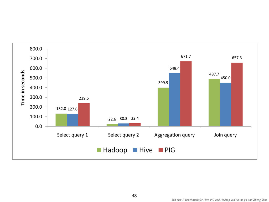
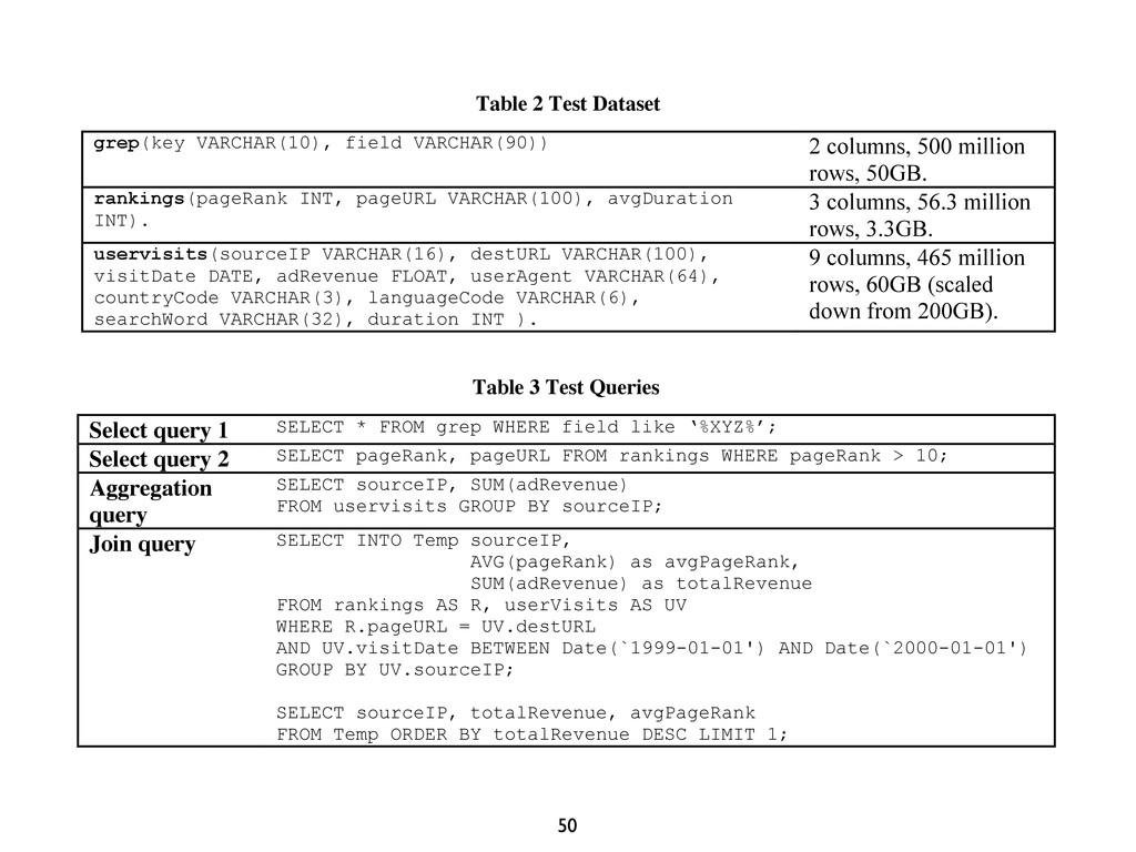
50. See Table 2 for more details about the data set. We tested the first four of the five queries, which include two select queries, one aggregation query and one join query4. We have reproduced the queries in Table 3. Details on how to generate the data can be found in the Hive benchmark package [6]. Table 2 Test Dataset grep(key VARCHAR(10), field VARCHAR(90)) 2 columns, 500 million rows, 50GB. rankings(pageRank INT, pageURL VARCHAR(100), avgDuration INT). 3 columns, 56.3 million rows, 3.3GB. uservisits(sourceIP VARCHAR(16), destURL VARCHAR(100), visitDate DATE, adRevenue FLOAT, userAgent VARCHAR(64), countryCode VARCHAR(3), languageCode VARCHAR(6), searchWord VARCHAR(32), duration INT ). 9 columns, 465 million rows, 60GB (scaled down from 200GB). Table 3 Test Queries Select query 1 SELECT  *  FROM  grep  WHERE  field  like  ‘%XYZ%’;; Select query 2 SELECT pageRank, pageURL FROM rankings WHERE pageRank > 10; Aggregation query SELECT sourceIP, SUM(adRevenue) FROM uservisits GROUP BY sourceIP; Join query SELECT INTO Temp sourceIP, AVG(pageRank) as avgPageRank, SUM(adRevenue) as totalRevenue FROM rankings AS R, userVisits AS UV WHERE R.pageURL = UV.destURL AND UV.visitDate BETWEEN Date(`1999-01-01') AND Date(`2000-01-01') GROUP BY UV.sourceIP; SELECT sourceIP, totalRevenue, avgPageRank FROM Temp ORDER BY totalRevenue DESC LIMIT 1; 3 Benchmark Results 50