Optimized Gravitational-wave Sky-mapping With Pulsar-timing Arrays

Contributed presentation for the NANOGrav Fall 2016 meeting at NCSA, University of Illinois at Urbana-Champaign.

Transcript

1. Stephen Taylor NANOGrav Fall Meeting, 10-21-2016 © 2016 California Institute of Technology. Government sponsorship acknowledged Stephen Taylor Optimized GW Sky-mapping With PTAs JET PROPULSION LABORATORY, CALIFORNIA INSTITUTE OF TECHNOLOGY
2. Stephen Taylor NANOGrav Fall Meeting, 10-21-2016 What can GW anisotropy tell us? Current techniques New trans-dimensional techniques, and model selection New techniques in action Overview
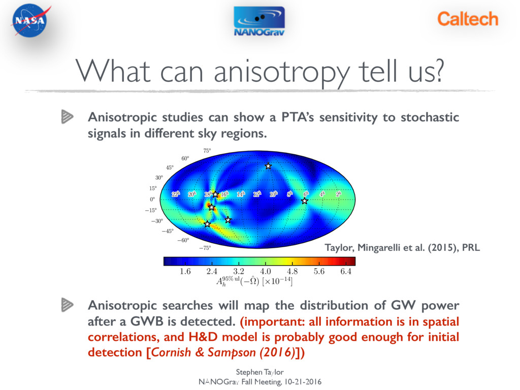
3. Stephen Taylor NANOGrav Fall Meeting, 10-21-2016 What can anisotropy tell us? Anisotropic studies can show a PTA’s sensitivity to stochastic signals in different sky regions. ! ! ! ! ! ! Anisotropic searches will map the distribution of GW power after a GWB is detected. (important: all information is in spatial correlations, and H&D model is probably good enough for initial detection [Cornish & Sampson (2016)]) 1.6 2.4 3.2 4.0 4.8 5.6 6.4 A95% ul h ( ˆ ⌦) [⇥10 14] Taylor, Mingarelli et al. (2015), PRL
4. Stephen Taylor NANOGrav Fall Meeting, 10-21-2016 What about science beyond detection! Sky power-mapping needs to dig into the spatial correlations. Search for single sources with power-mapping (more on this later). Matching the GWB distribution to galaxy distributions. Alternatively, use galaxy maps as priors [e.g. Chiara’s project]. What can anisotropy tell us?
5. Stephen Taylor NANOGrav Fall Meeting, 10-21-2016 Current techniques
6. Stephen Taylor NANOGrav Fall Meeting, 10-21-2016 Current techniques ab / (1 + ab) Z d2 ˆ ⌦P(ˆ ⌦) h F(ˆ ⌦)+ a F(ˆ ⌦)+ b + F(ˆ ⌦)⇥ a F(ˆ ⌦)⇥ b i
7. Stephen Taylor NANOGrav Fall Meeting, 10-21-2016 Current techniques ab / (1 + ab) Z d2 ˆ ⌦P(ˆ ⌦) h F(ˆ ⌦)+ a F(ˆ ⌦)+ b + F(ˆ ⌦)⇥ a F(ˆ ⌦)⇥ b i Gair, Romano, Taylor, Mingarelli (2014)
8. Stephen Taylor NANOGrav Fall Meeting, 10-21-2016 Current techniques ab / (1 + ab) Z d2 ˆ ⌦P(ˆ ⌦) h F(ˆ ⌦)+ a F(ˆ ⌦)+ b + F(ˆ ⌦)⇥ a F(ˆ ⌦)⇥ b i Gair, Romano, Taylor, Mingarelli (2014)
9. Stephen Taylor NANOGrav Fall Meeting, 10-21-2016 Current techniques ab / (1 + ab) Z d2 ˆ ⌦P(ˆ ⌦) h F(ˆ ⌦)+ a F(ˆ ⌦)+ b + F(ˆ ⌦)⇥ a F(ˆ ⌦)⇥ b i
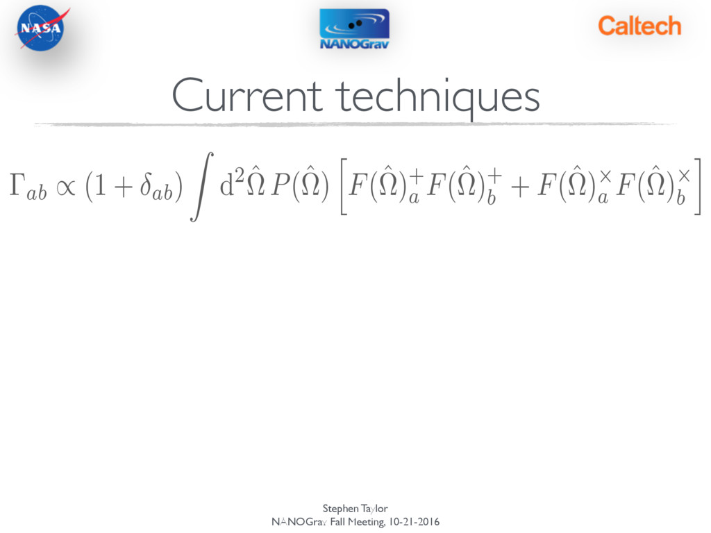
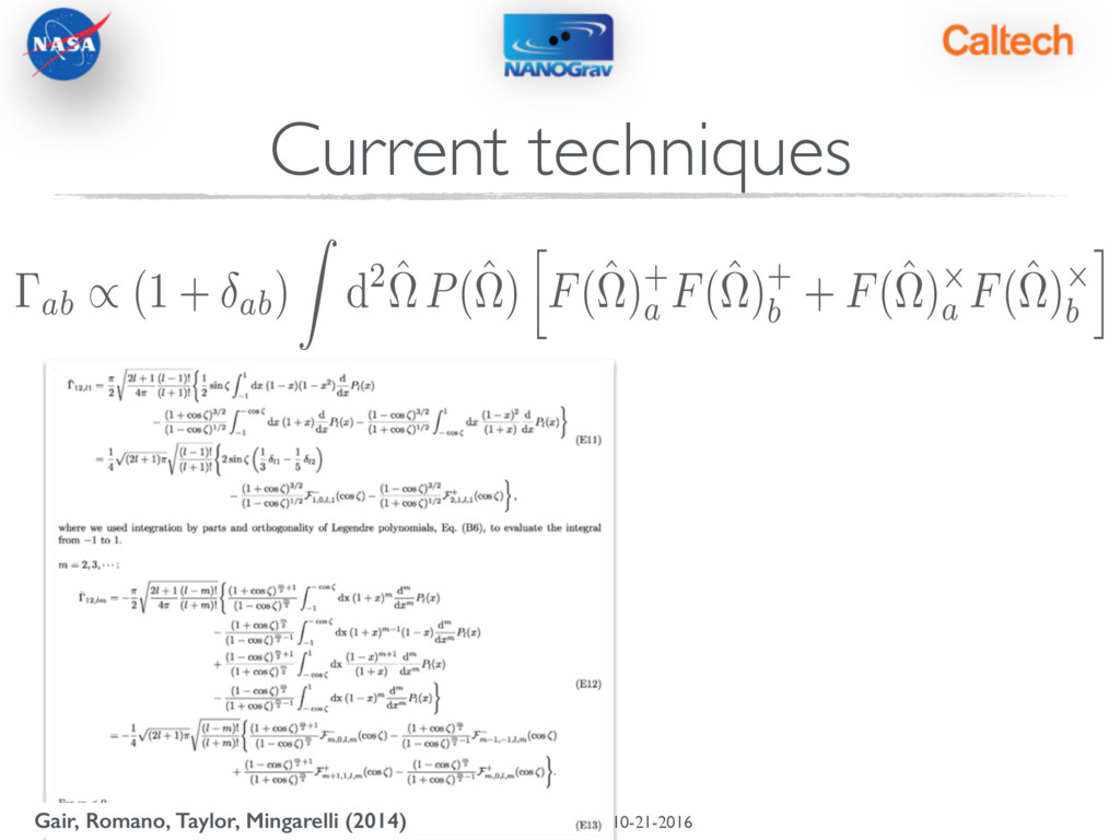
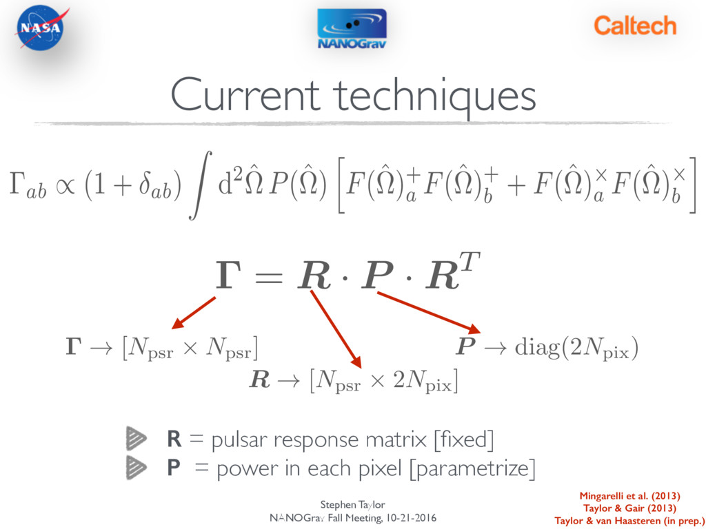
10. Stephen Taylor NANOGrav Fall Meeting, 10-21-2016 Current techniques R = pulsar response matrix [fixed] P = power in each pixel [parametrize] ab / (1 + ab) Z d2 ˆ ⌦P(ˆ ⌦) h F(ˆ ⌦)+ a F(ˆ ⌦)+ b + F(ˆ ⌦)⇥ a F(ˆ ⌦)⇥ b i = R · P · RT R ! [N psr ⇥ 2N pix ] P ! diag(2N pix ) ! [Npsr ⇥ Npsr] Mingarelli et al. (2013) Taylor & Gair (2013) Taylor & van Haasteren (in prep.)
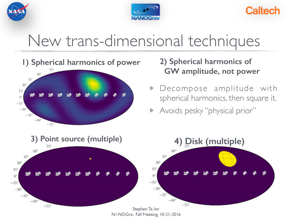
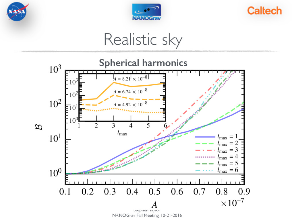
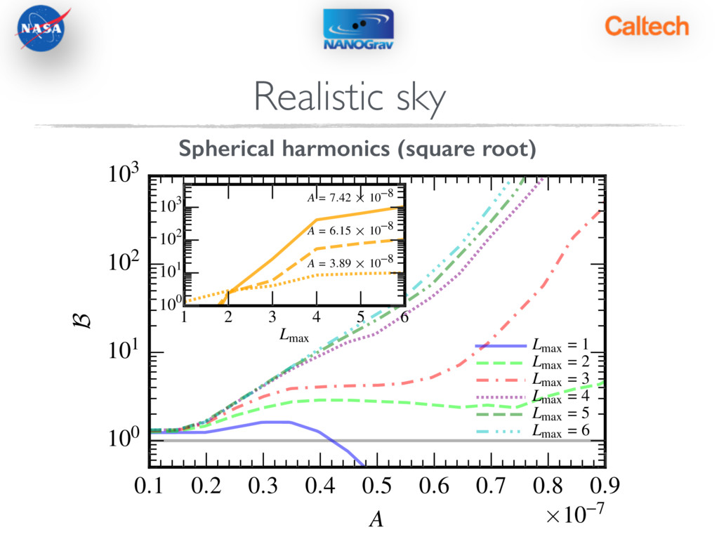
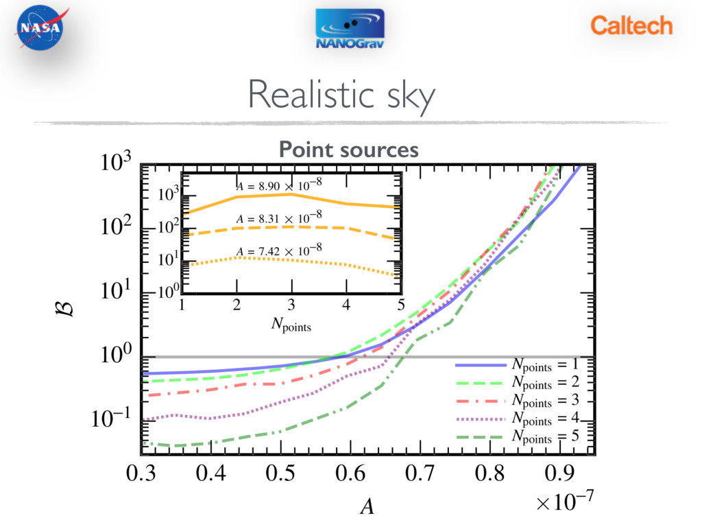
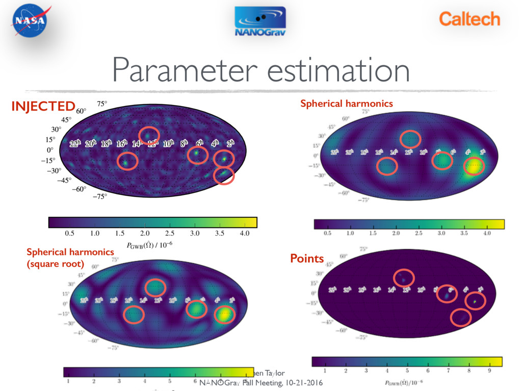
11. Stephen Taylor NANOGrav Fall Meeting, 10-21-2016 New trans-dimensional techniques 1) Spherical harmonics of power 4) Disk (multiple) 3) Point source (multiple) 2) Spherical harmonics of GW amplitude, not power Decompose amplitude with spherical harmonics, then square it. Avoids pesky “physical prior”
12. Stephen Taylor NANOGrav Fall Meeting, 10-21-2016 New trans-dimensional techniques In all cases, we let the data decide how anisotropic our model should be. Let Bayesian model selection select optimal degree of anisotropy (spherical harmonic “ ”), number of point sources, or number of hotspots. Throw in spherical harmonics, points, and hotspots together, and let the data sort it all out! l
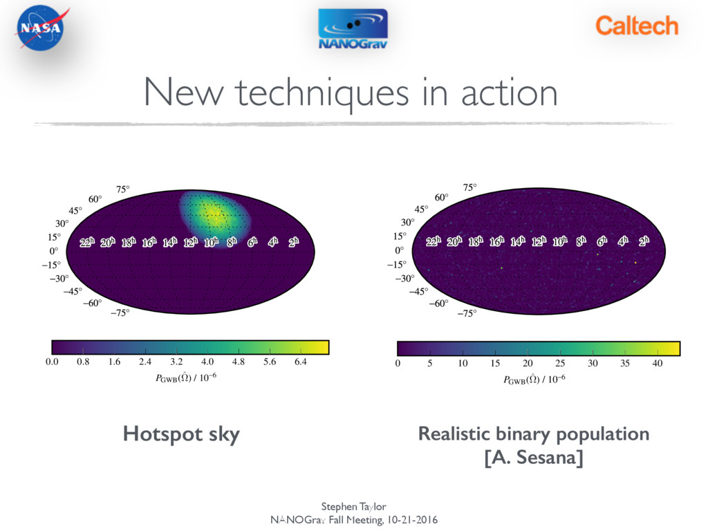
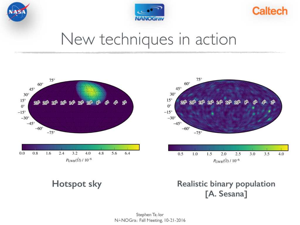
13. Stephen Taylor NANOGrav Fall Meeting, 10-21-2016 Simple injection and recovery program to test relative efficacy of different techniques on different skies. No need for timing model, or even a red GWB spectrum. These would add realism, but won’t affect qualitative results. Run MCMC over parameters and models (using product-space sampling). New techniques in action
14. Stephen Taylor NANOGrav Fall Meeting, 10-21-2016 0 5 10 15 20 25 30 35 40 PGWB(ˆ ⌦) / 10-6 0.0 0.8 1.6 2.4 3.2 4.0 4.8 5.6 6.4 PGWB(ˆ ⌦) / 10-6 New techniques in action Hotspot sky Realistic binary population [A. Sesana]
15. Stephen Taylor NANOGrav Fall Meeting, 10-21-2016 0 5 10 15 20 25 30 35 40 PGWB(ˆ ⌦) / 10-6 0.0 0.8 1.6 2.4 3.2 4.0 4.8 5.6 6.4 PGWB(ˆ ⌦) / 10-6 0.5 1.0 1.5 2.0 2.5 3.0 3.5 4.0 PGWB(ˆ ⌦) / 10-6 New techniques in action Hotspot sky Realistic binary population [A. Sesana]
16. Stephen Taylor NANOGrav Fall Meeting, 10-21-2016 Realistic sky 0.1 0.2 0.3 0.4 0.5 0.6 0.7 0.8 0.9 A ⇥10-7 100 101 102 103 B lmax = 1 lmax = 2 lmax = 3 lmax = 4 lmax = 5 lmax = 6 1 2 3 4 5 6 lmax 100 101 102 103 A = 4.92 ⇥ 10-8 A = 6.74 ⇥ 10-8 A = 8.21 ⇥ 10-8 Spherical harmonics
17. Stephen Taylor NANOGrav Fall Meeting, 10-21-2016 Realistic sky Spherical harmonics (square root) 0.1 0.2 0.3 0.4 0.5 0.6 0.7 0.8 0.9 A ⇥10-7 100 101 102 103 B Lmax = 1 Lmax = 2 Lmax = 3 Lmax = 4 Lmax = 5 Lmax = 6 1 2 3 4 5 6 Lmax 100 101 102 103 A = 3.89 ⇥ 10-8 A = 6.15 ⇥ 10-8 A = 7.42 ⇥ 10-8
18. Stephen Taylor NANOGrav Fall Meeting, 10-21-2016 Realistic sky 0.3 0.4 0.5 0.6 0.7 0.8 0.9 A ⇥10-7 10-1 100 101 102 103 B Npoints = 1 Npoints = 2 Npoints = 3 Npoints = 4 Npoints = 5 1 2 3 4 5 Npoints 100 101 102 103 A = 7.42 ⇥ 10-8 A = 8.31 ⇥ 10-8 A = 8.90 ⇥ 10-8 Point sources
19. Stephen Taylor NANOGrav Fall Meeting, 10-21-2016 Sky recovery 0.5 1.0 1.5 2.0 2.5 3.0 3.5 4.0 PGWB(ˆ ⌦) / 10-6 Spherical harmonics Spherical harmonics (square root) Points Parameter estimation INJECTED
20. Stephen Taylor NANOGrav Fall Meeting, 10-21-2016 Summary GW sky may be dominated by a few bright sources, clustered sources, or may be relatively smooth. Ultimately, the pulsar-timing data will tell us which. We have fast, flexible models to probe the spatial correlations between pulsars. These can infer the optimal description of the GW sky, whether as a collection of points, spherical harmonics, or hotspots. All techniques can be readily implemented on real data with NX01 (https://github.com/stevertaylor/NX01).