Slides presented at my lab about Introduction to LP-MERT (Galley & Quirk, EMNLP 2011), which is an exact search algorithm for minimum error rate training for statistical machine translation.
Chris Quirk EMNLP 2011 Presenter: Tetsuo Kiso MT study group meeting November 22, 2012 Feel free to email me if these slide contains any mistakes! [email protected] Thursday, November 29, 12
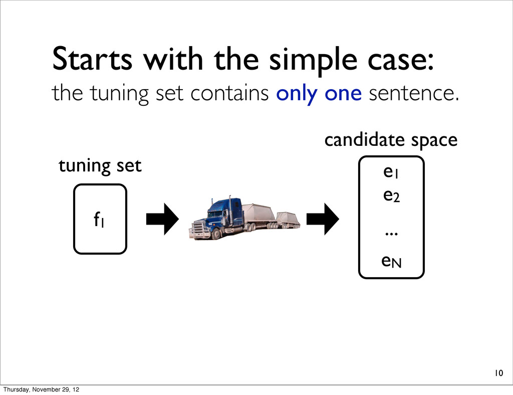
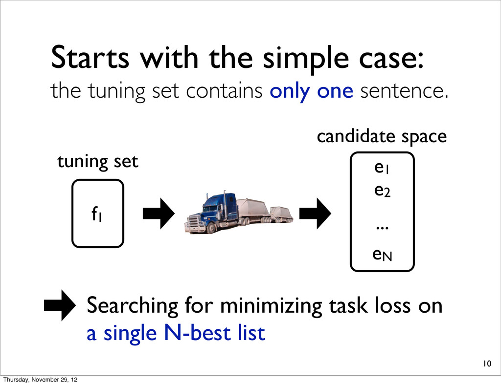
common practice: parameters are tuned using MERT on a small development set image url: http://wyofile.com/wp-content/uploads/2010/11/chiefjoe-haultruck.jpg moses parallel corpus monolingual corpus Thursday, November 29, 12
• directly optimizes the evaluation metric - e.g., BLEU (Papineni+, 2002), TER (Snover+, 2006) • originally from speech recognition (as always) • Typically, search space is approximated by N- best lists - Extensions: lattice MERT (Macherey+, 2008), hypergraph MERT (Kumar+, 2009) 4 Thursday, November 29, 12
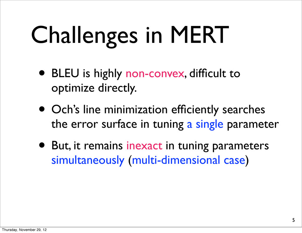
optimize directly. • Och’s line minimization efficiently searches the error surface in tuning a single parameter • But, it remains inexact in tuning parameters simultaneously (multi-dimensional case) 5 Thursday, November 29, 12
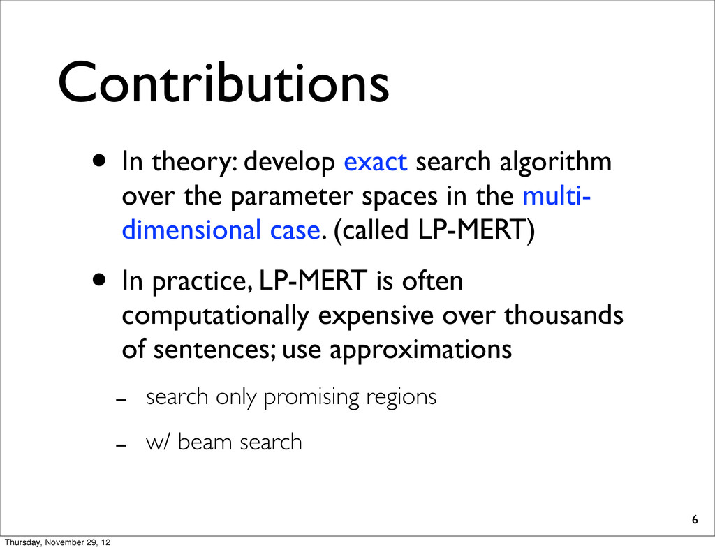
parameter spaces in the multi- dimensional case. (called LP-MERT) • In practice, LP-MERT is often computationally expensive over thousands of sentences; use approximations - search only promising regions - w/ beam search 6 Thursday, November 29, 12
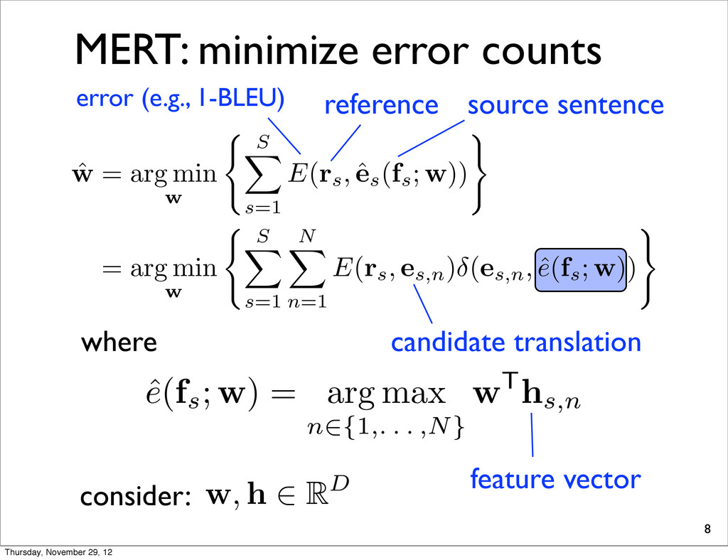
w ( S X s=1 E(rs, ˆ es(fs; w)) ) = arg min w ( S X s=1 N X n=1 E(rs, es,n) (es,n, ˆ e(fs; w)) ) ˆ e ( fs; w ) = arg max n2{1,. . . ,N} wThs,n where reference candidate translation source sentence error (e.g., 1-BLEU) feature vector w, h 2 RD consider: Thursday, November 29, 12
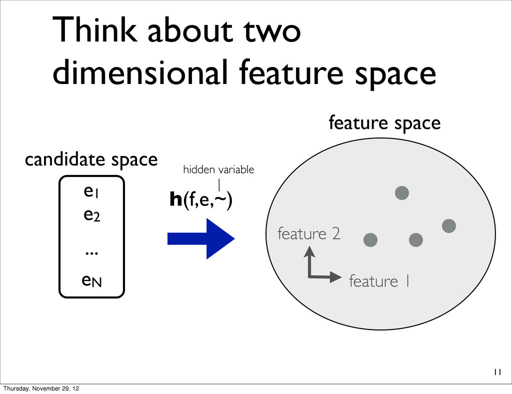
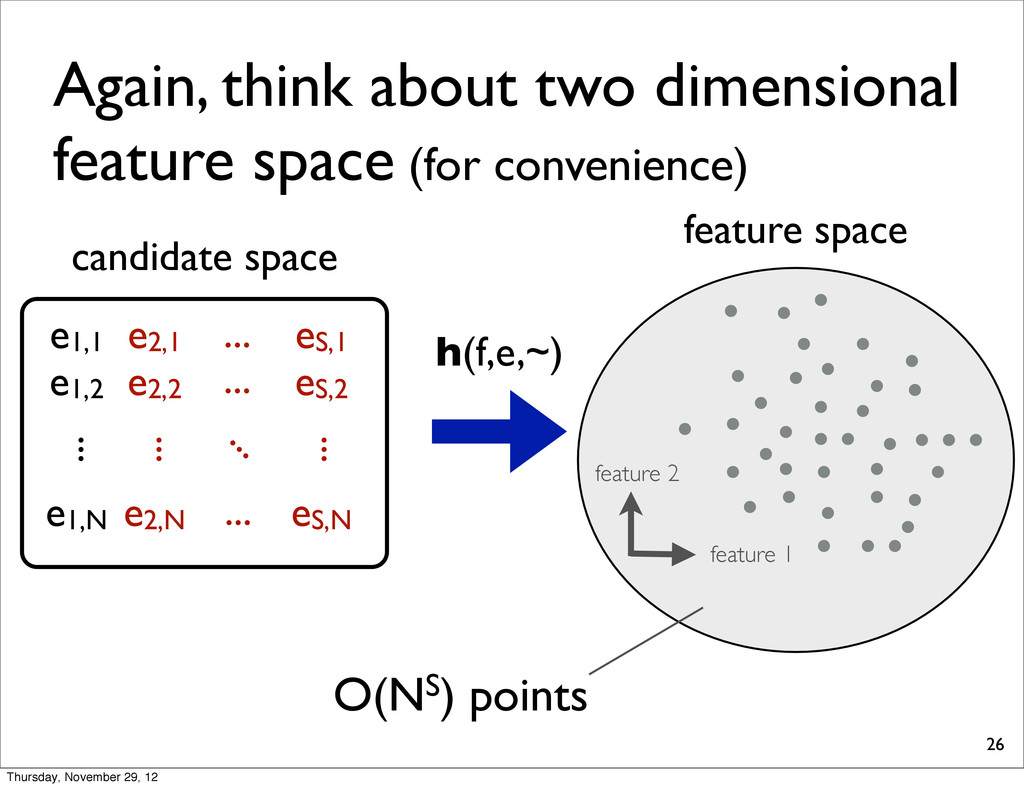
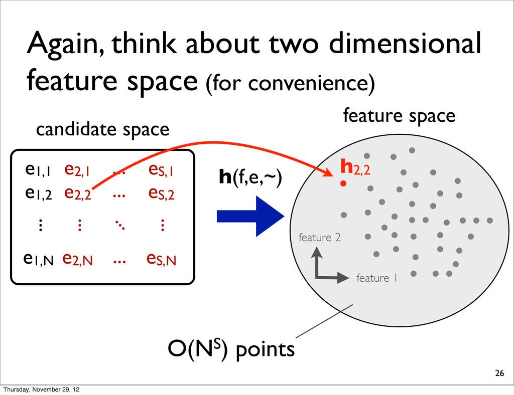
1 feature 2 candidate space e1 e2 eN ... h(f,e,~) h2(e2) feature space each point corresponds to a feature vector for each translation Thursday, November 29, 12
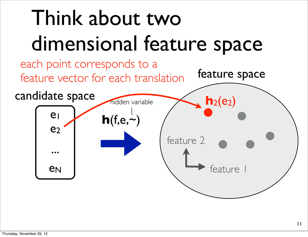
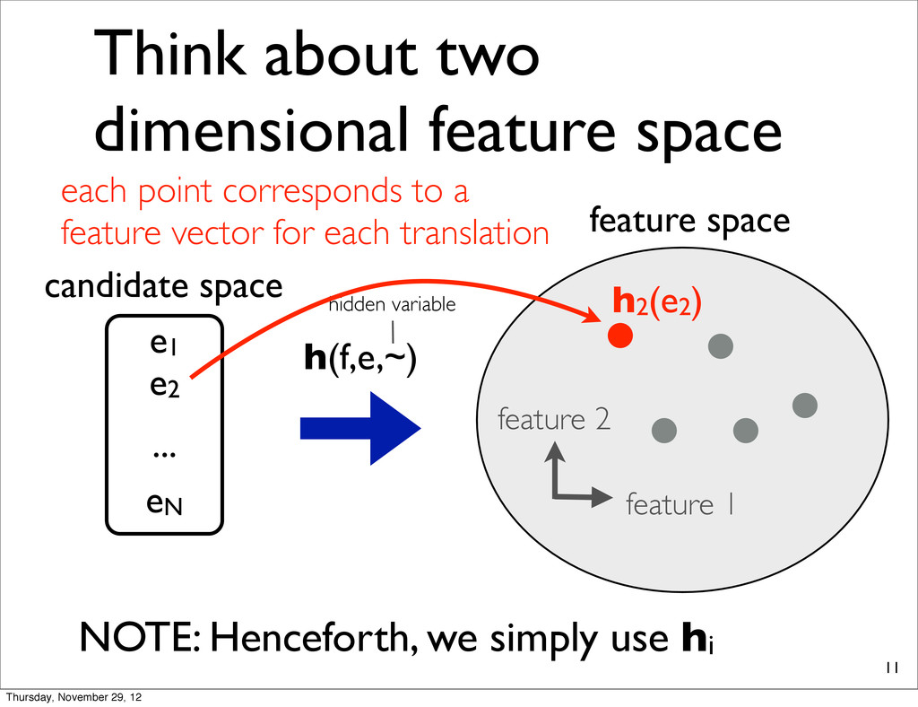
1 feature 2 candidate space e1 e2 eN ... h(f,e,~) h2(e2) feature space NOTE: Henceforth, we simply use hi each point corresponds to a feature vector for each translation Thursday, November 29, 12
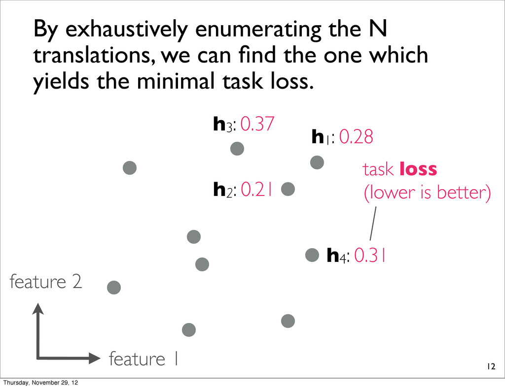
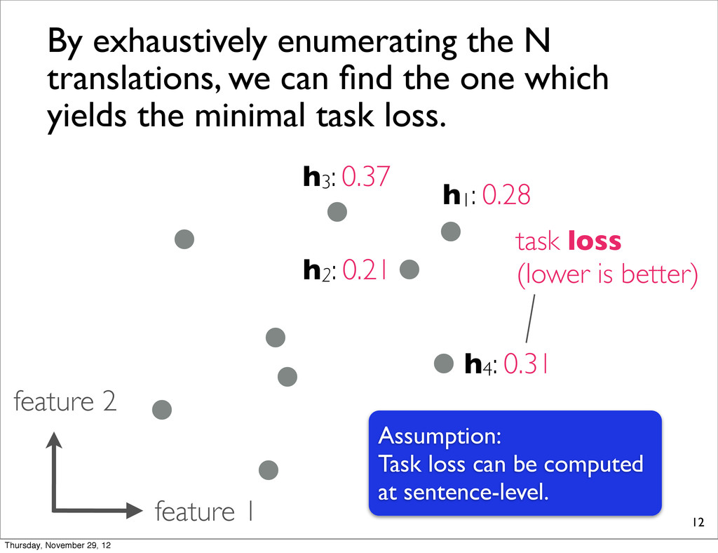
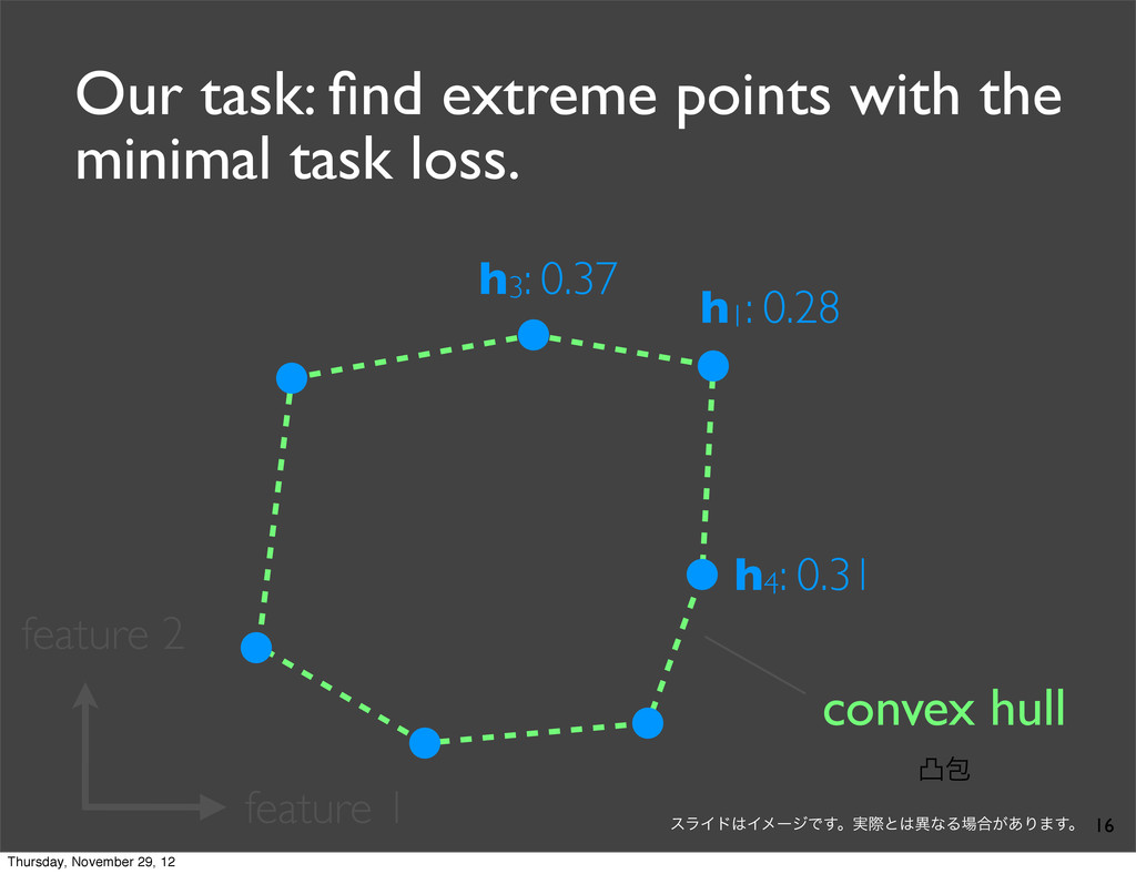
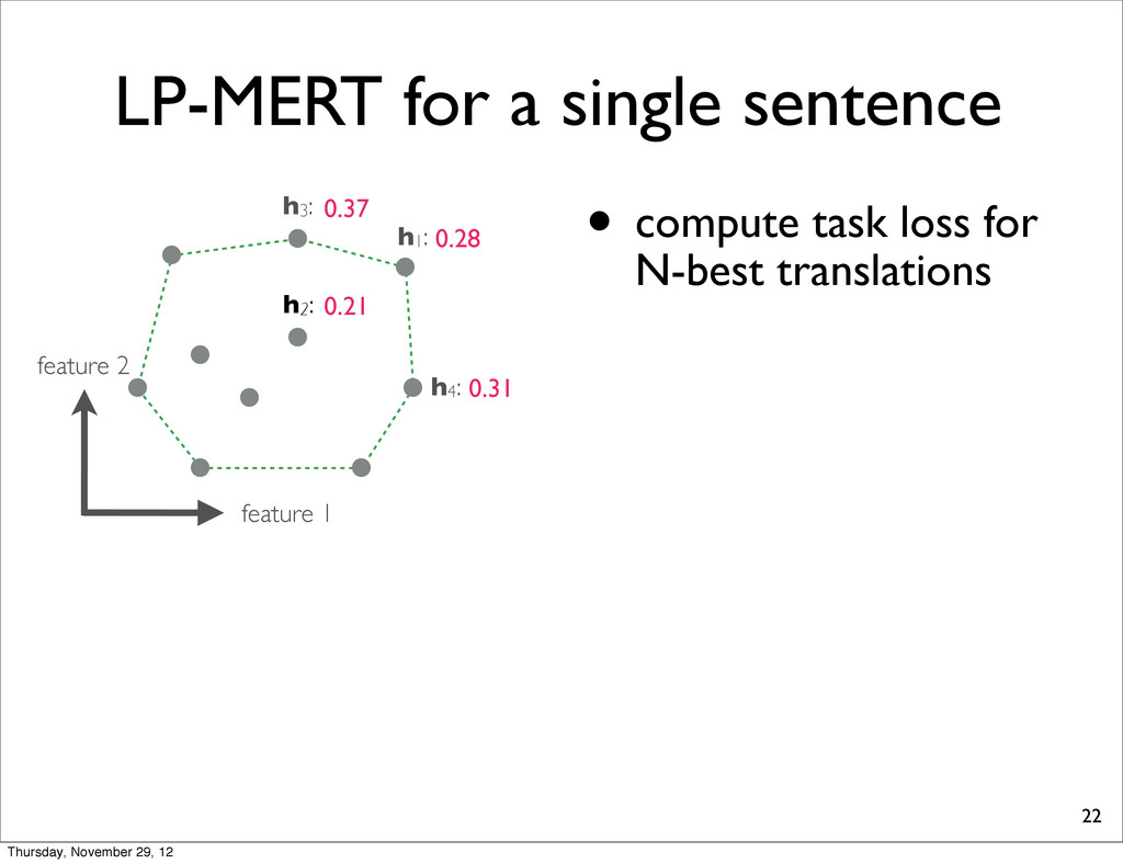
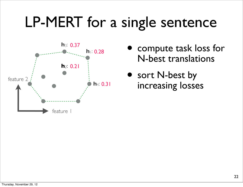
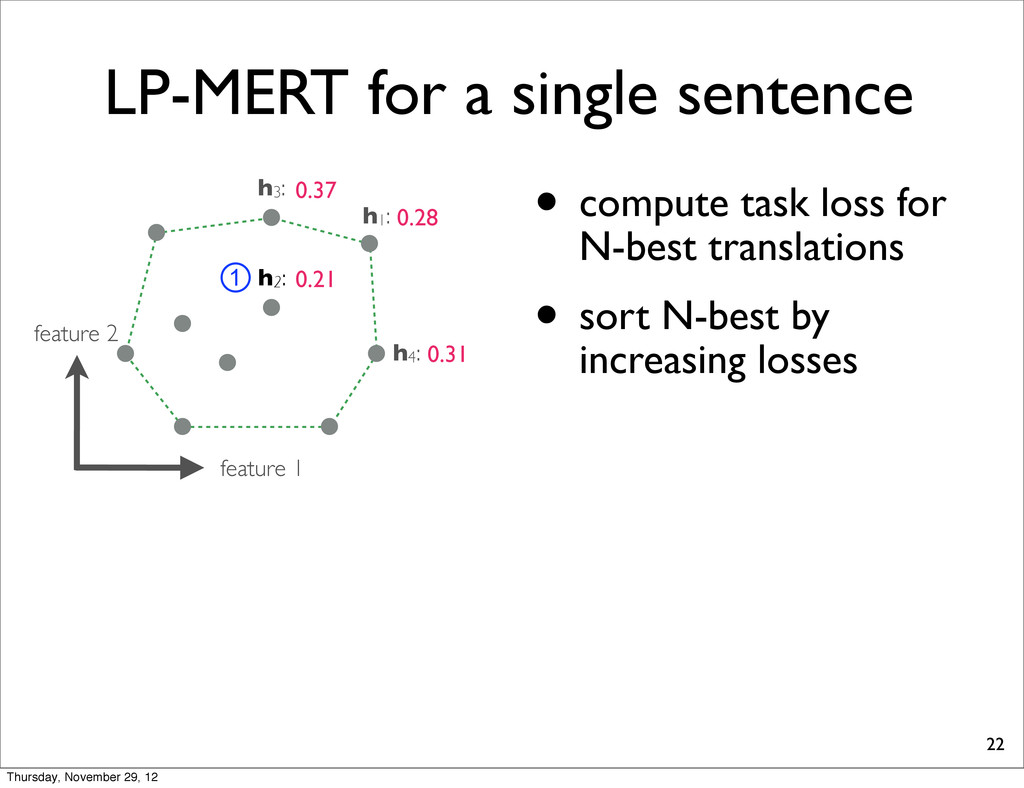
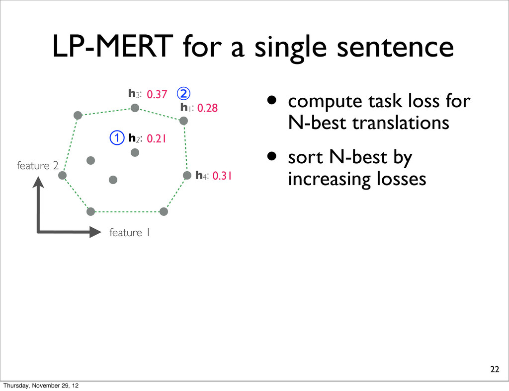
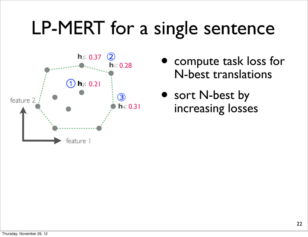
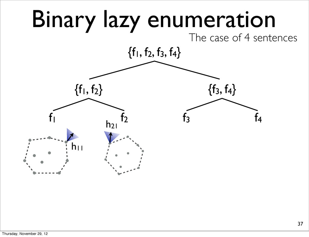
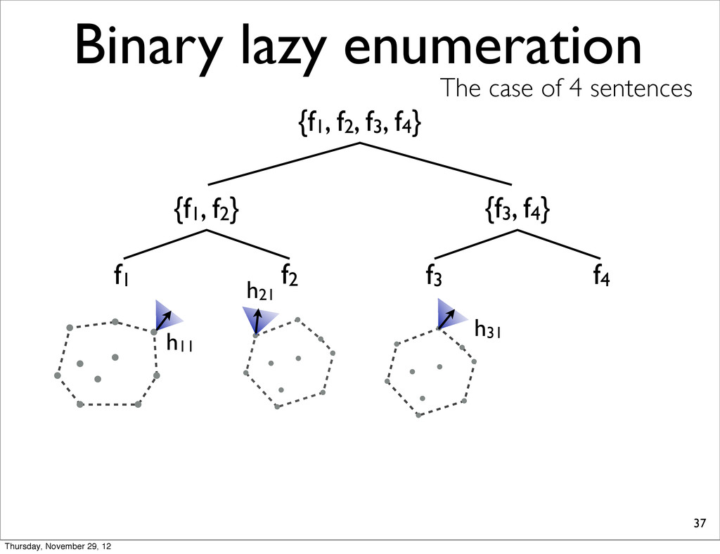
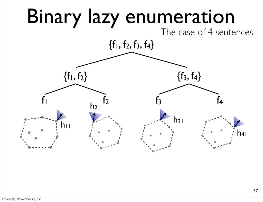
0.37 h4: 0.31 task loss (lower is better) By exhaustively enumerating the N translations, we can find the one which yields the minimal task loss. Thursday, November 29, 12
0.37 h4: 0.31 task loss (lower is better) By exhaustively enumerating the N translations, we can find the one which yields the minimal task loss. Assumption: Task loss can be computed at sentence-level. Thursday, November 29, 12
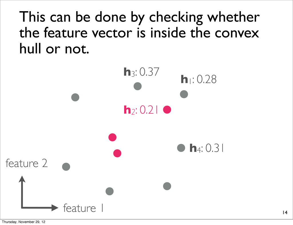
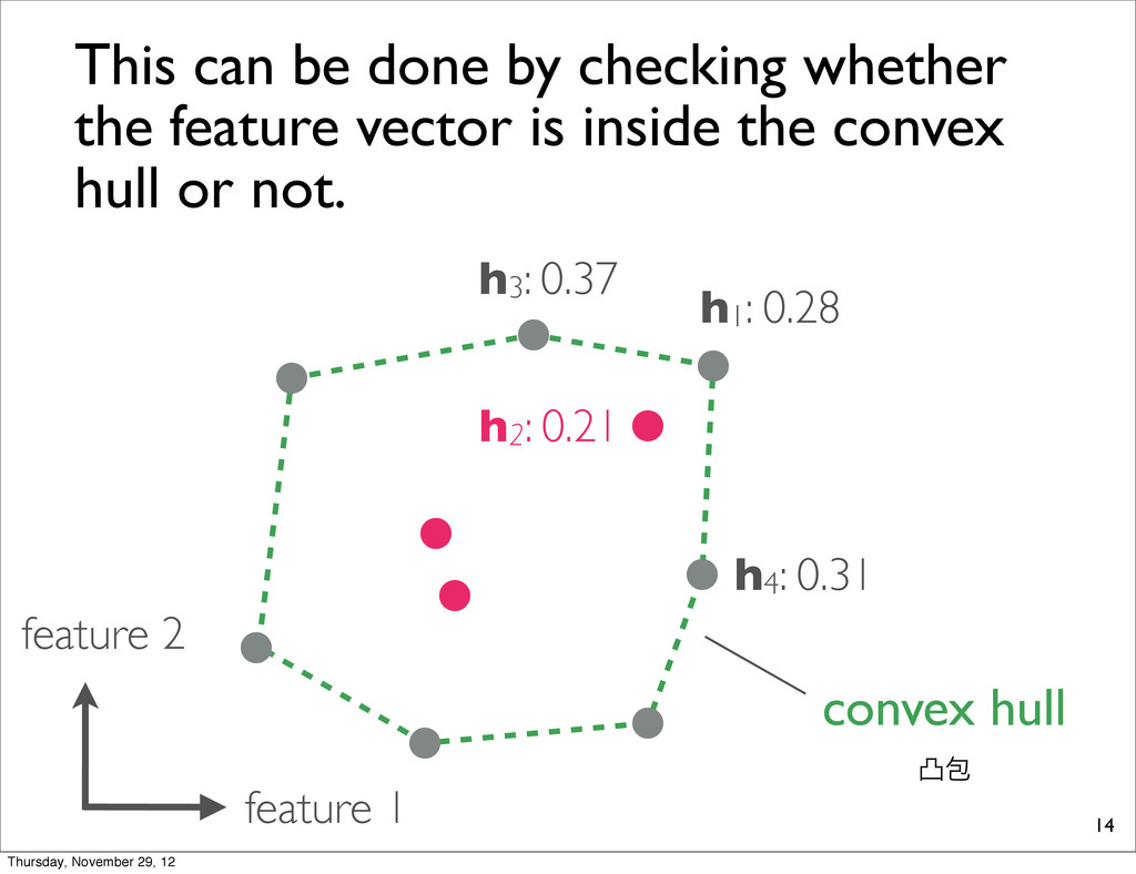
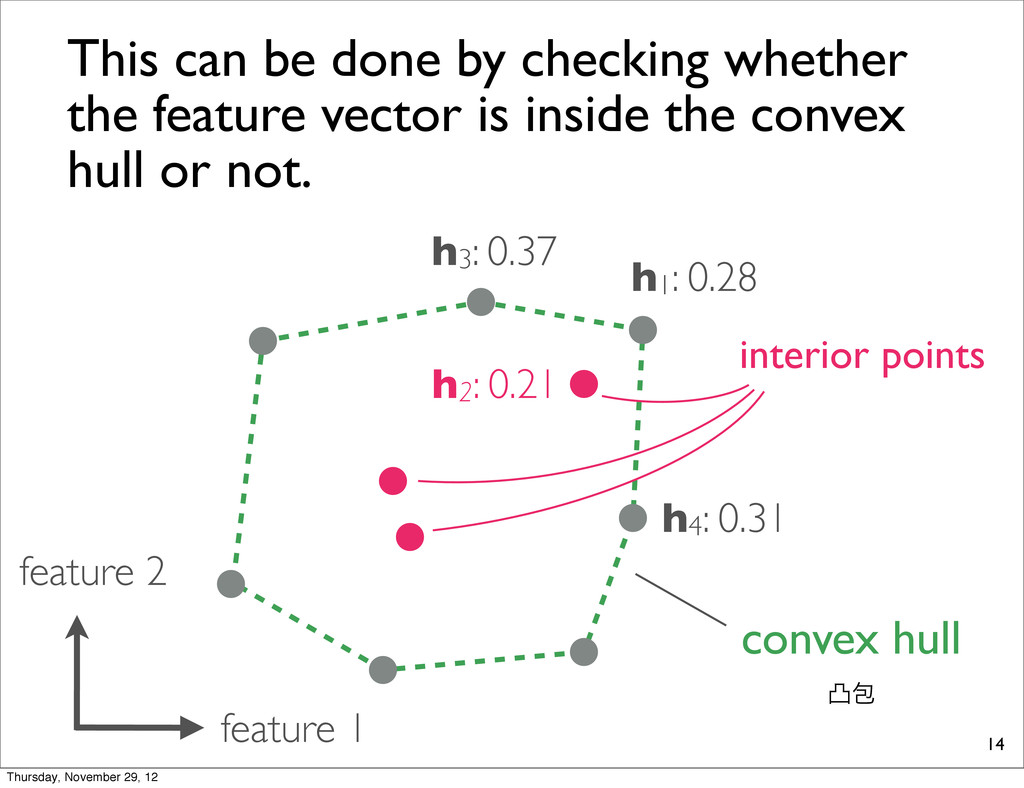
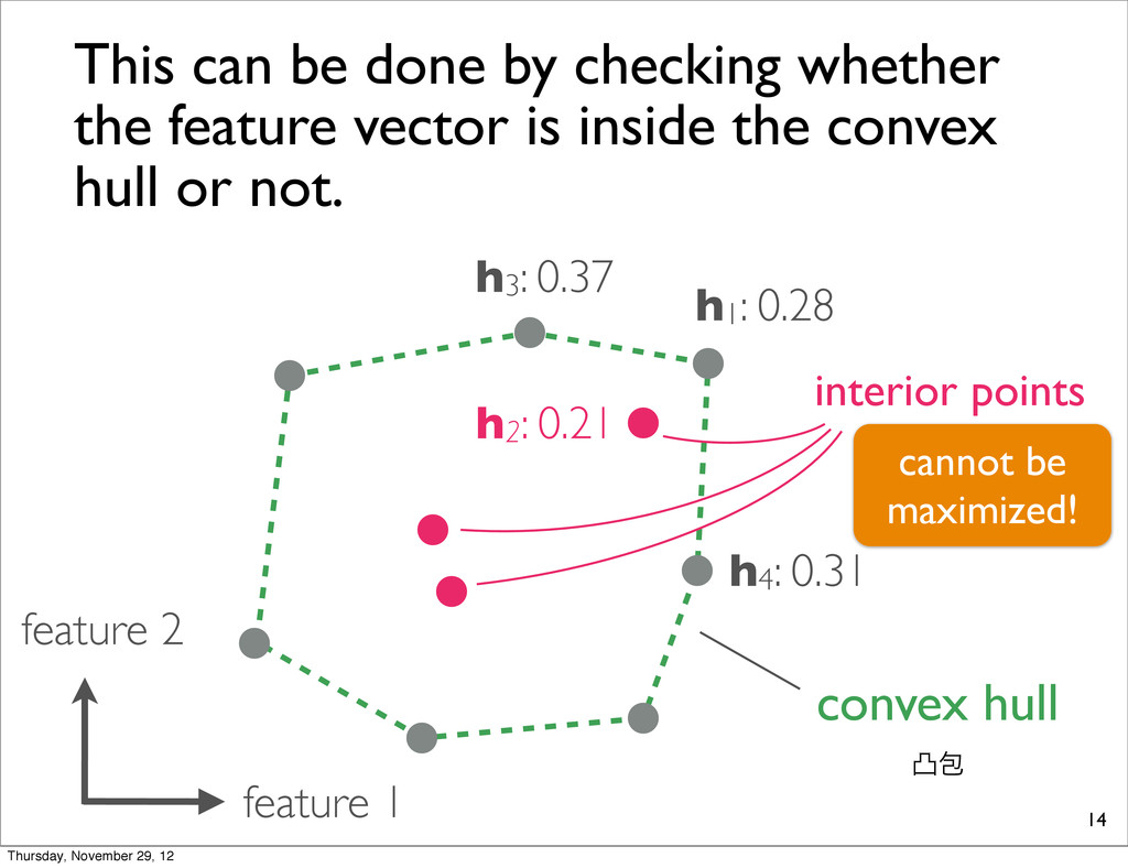
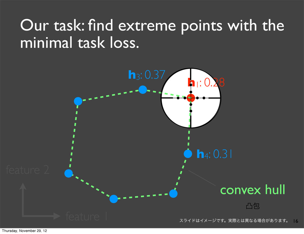
0.21 h3: 0.37 This can be done by checking whether the feature vector is inside the convex hull or not. convex hull ತแ interior points Thursday, November 29, 12
0.21 h3: 0.37 This can be done by checking whether the feature vector is inside the convex hull or not. convex hull ತแ interior points cannot be maximized! Thursday, November 29, 12
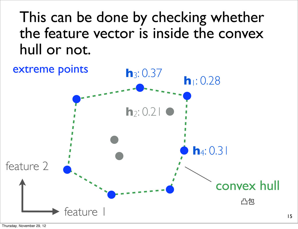
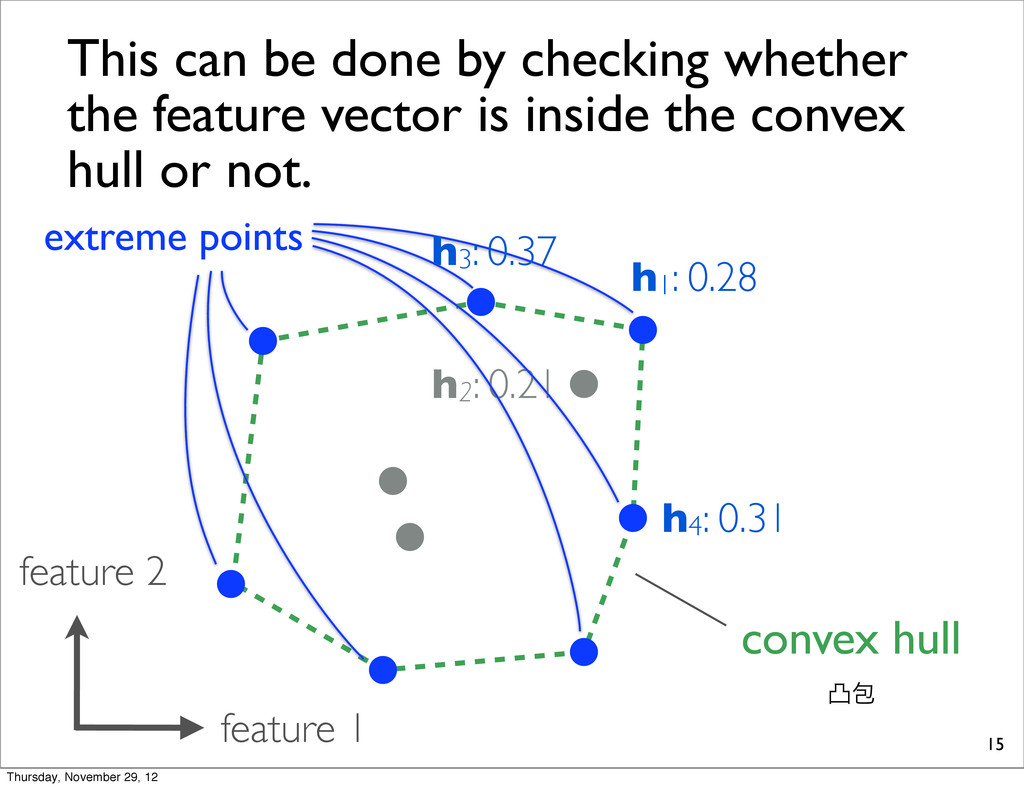
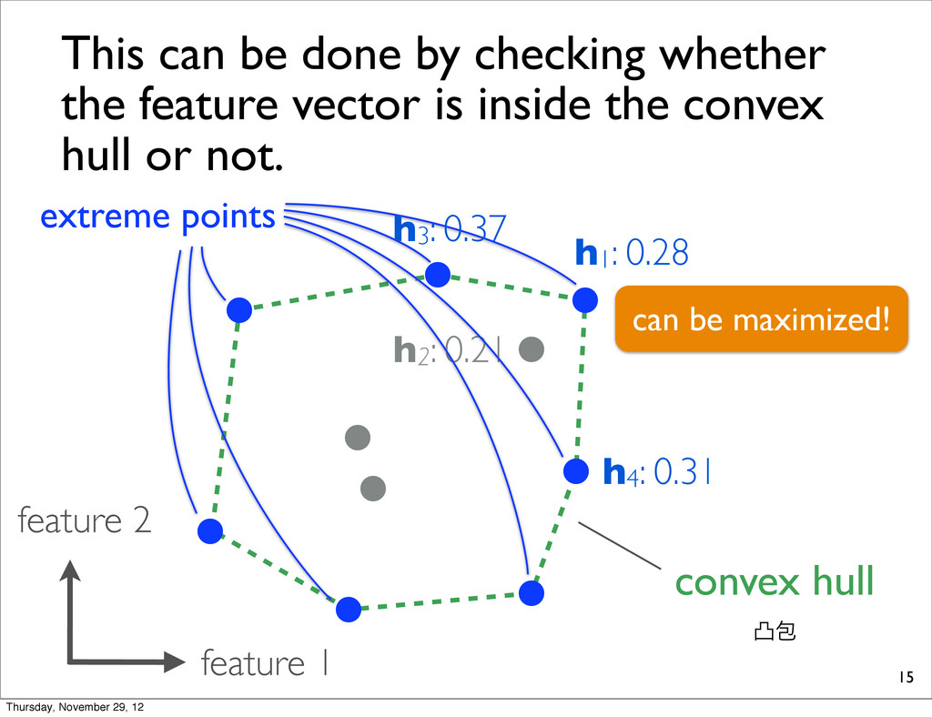
0.28 h3: 0.37 This can be done by checking whether the feature vector is inside the convex hull or not. convex hull ತแ extreme points Thursday, November 29, 12
0.28 h3: 0.37 This can be done by checking whether the feature vector is inside the convex hull or not. convex hull ತแ extreme points Thursday, November 29, 12
0.28 h3: 0.37 This can be done by checking whether the feature vector is inside the convex hull or not. convex hull ತแ extreme points can be maximized! Thursday, November 29, 12
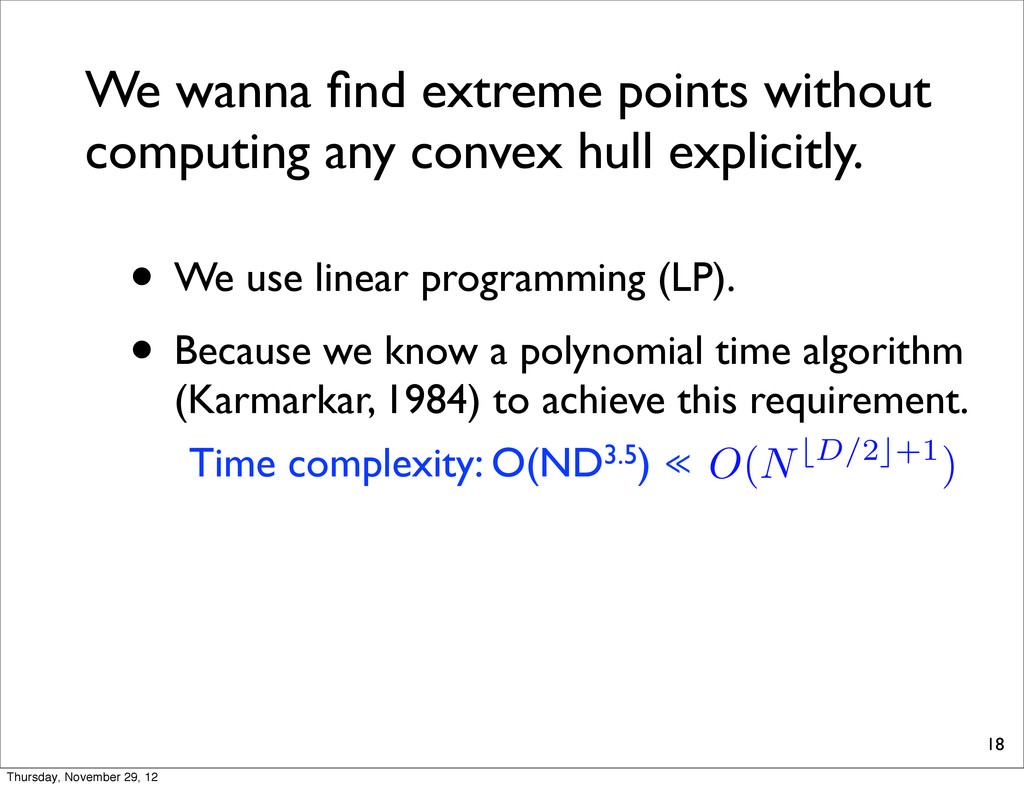
1977; Barber+, 1996) • Once we construct the convex hull, we can find the extreme points with the lowest loss! 17 This does not scale! Computing convex hull is very expensive! Thursday, November 29, 12
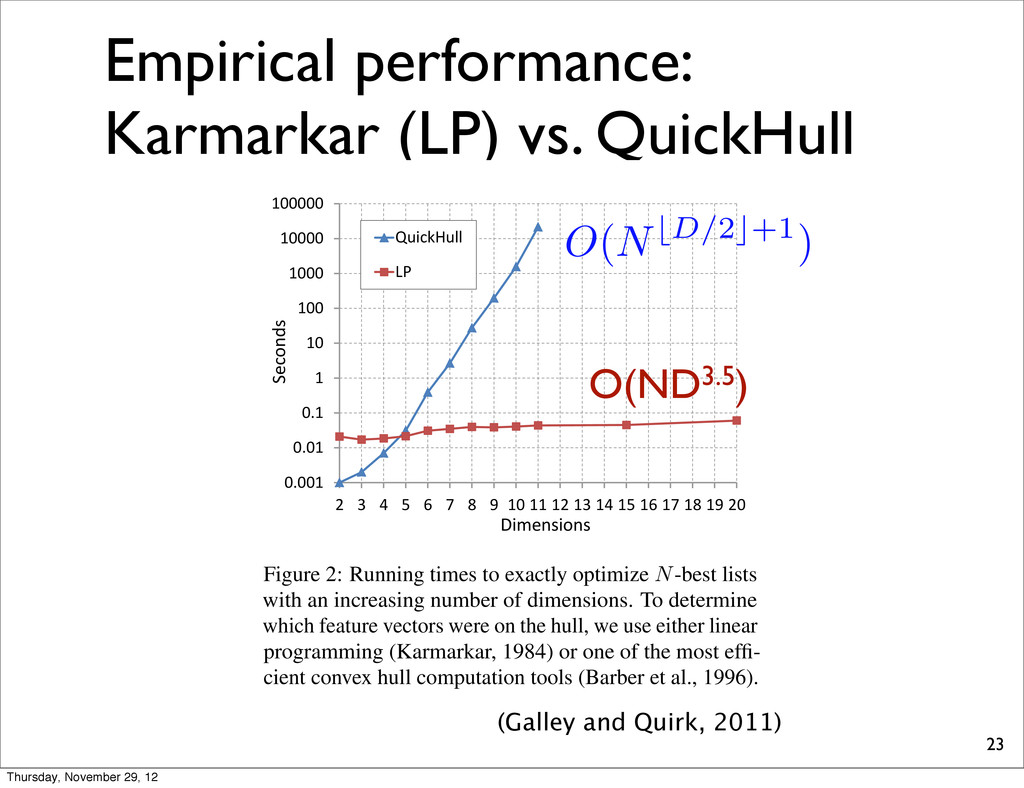
1977; Barber+, 1996) • Once we construct the convex hull, we can find the extreme points with the lowest loss! 17 Time complexity of the best known convex hull algorithm (Barber+, 1996): O(NbD/2c+1) This does not scale! Computing convex hull is very expensive! Thursday, November 29, 12
explicitly. • We use linear programming (LP). • Because we know a polynomial time algorithm (Karmarkar, 1984) to achieve this requirement. 18 Time complexity: O(ND3.5) ≪ O(NbD/2c+1) Thursday, November 29, 12
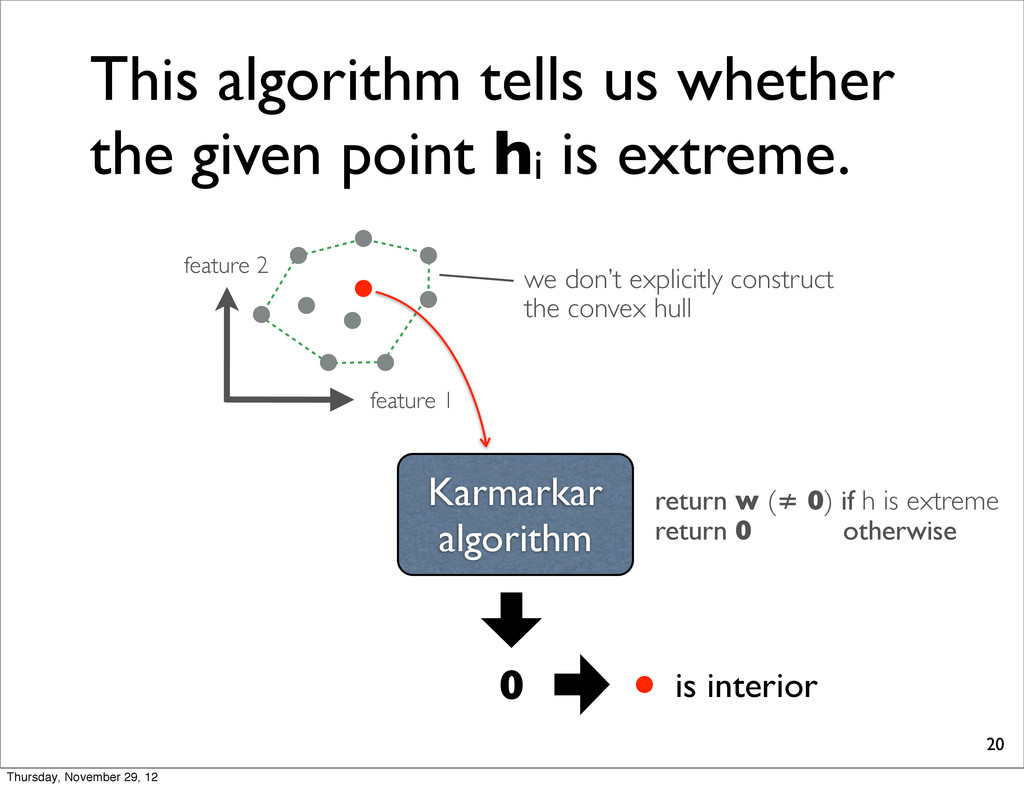
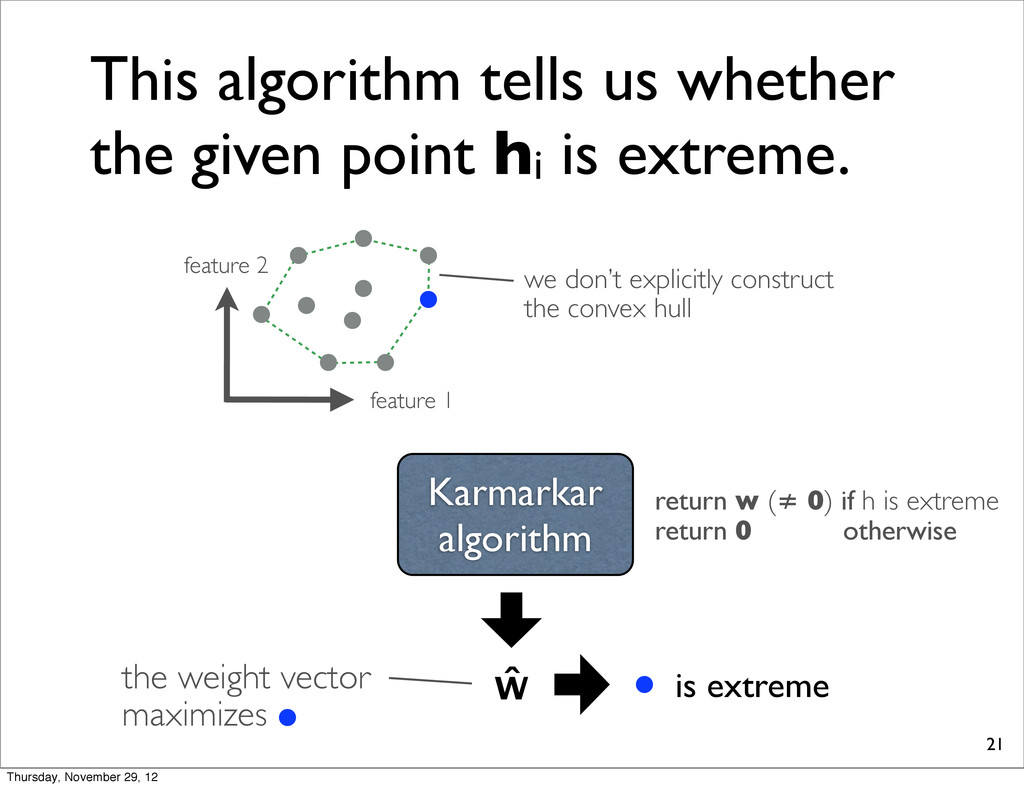
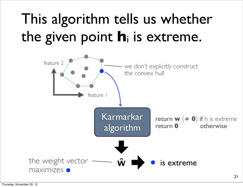
is extreme. Karmarkar algorithm feature 1 feature 2 we don’t explicitly construct the convex hull 0 return w (≠ 0) if h is extreme return 0 otherwise is interior Thursday, November 29, 12
is extreme. Karmarkar algorithm feature 1 feature 2 we don’t explicitly construct the convex hull ŵ return w (≠ 0) if h is extreme return 0 otherwise is extreme the weight vector maximizes Thursday, November 29, 12
is extreme. Karmarkar algorithm feature 1 feature 2 we don’t explicitly construct the convex hull ŵ return w (≠ 0) if h is extreme return 0 otherwise is extreme the weight vector maximizes Thursday, November 29, 12
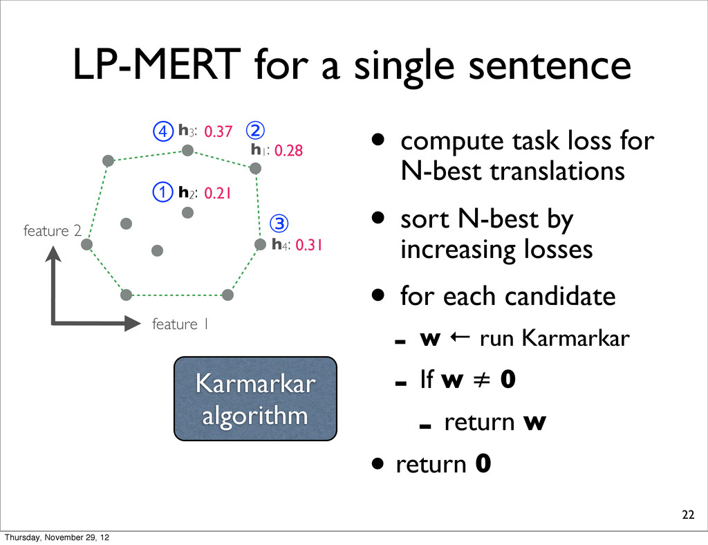
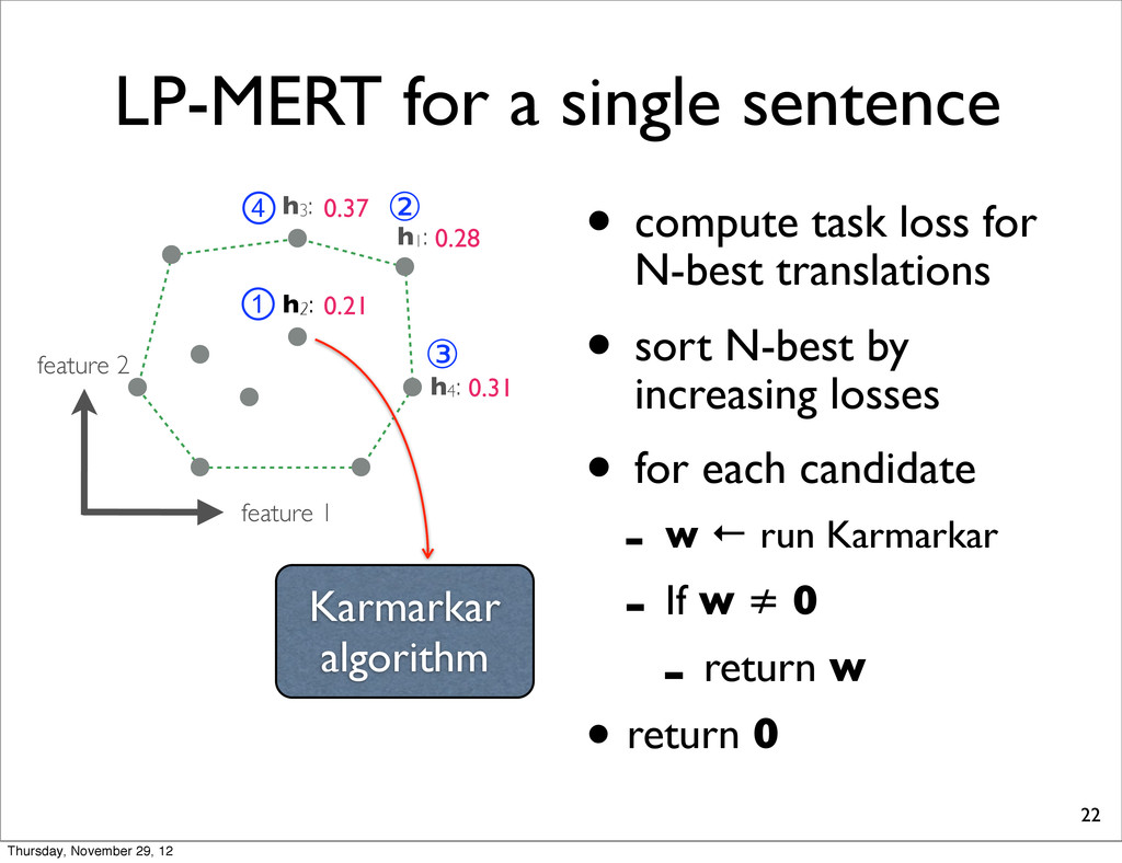
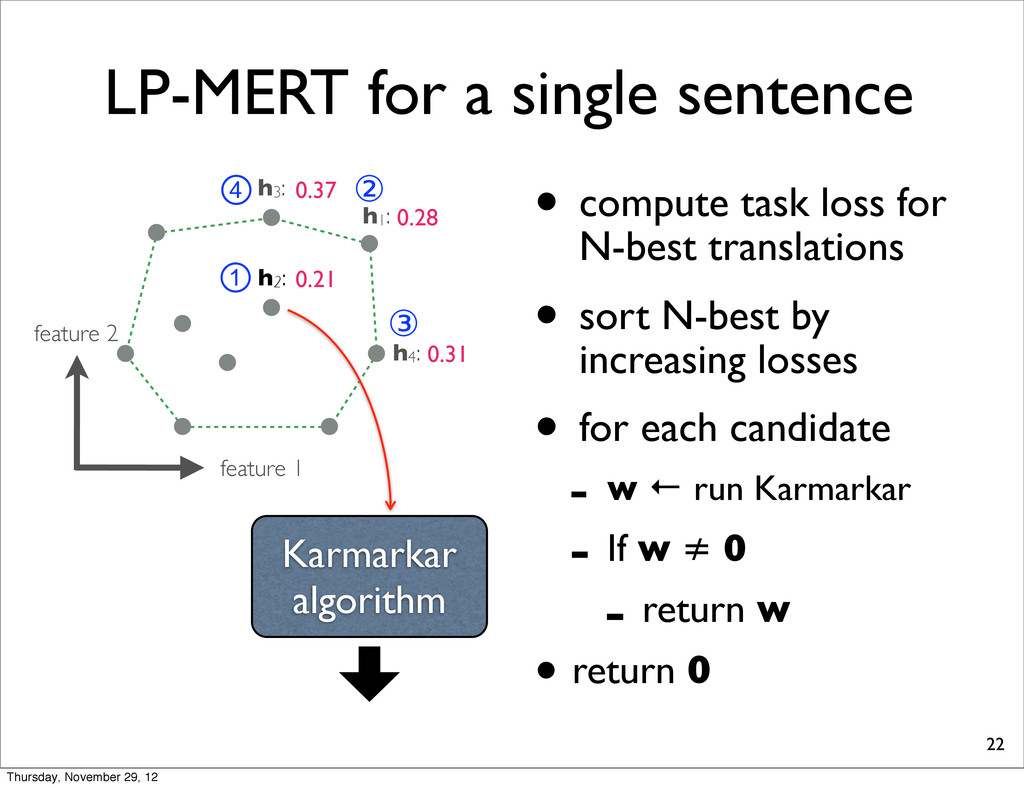
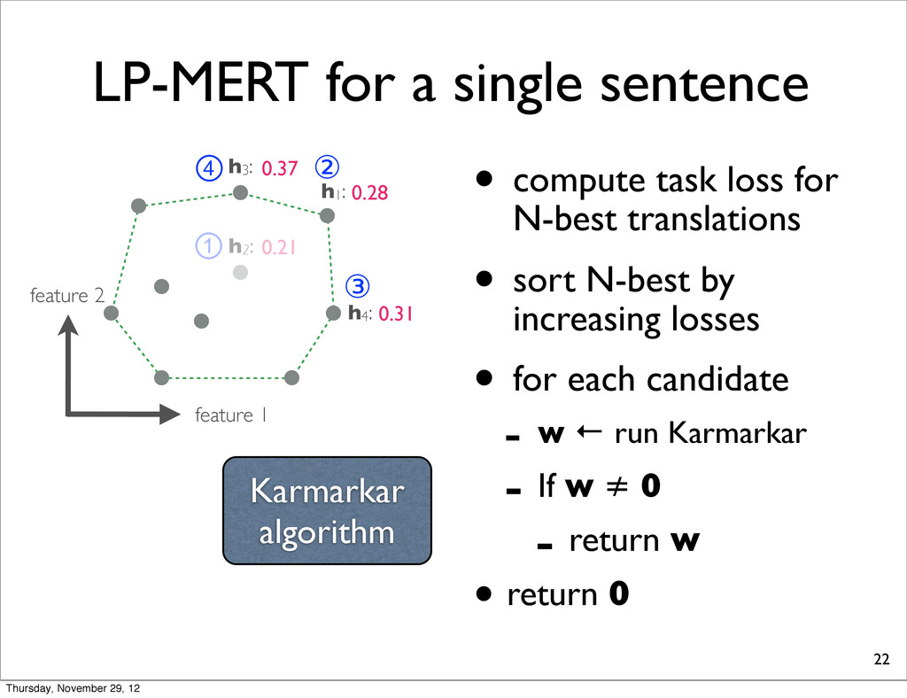
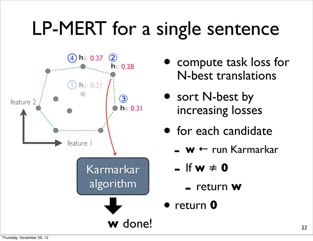
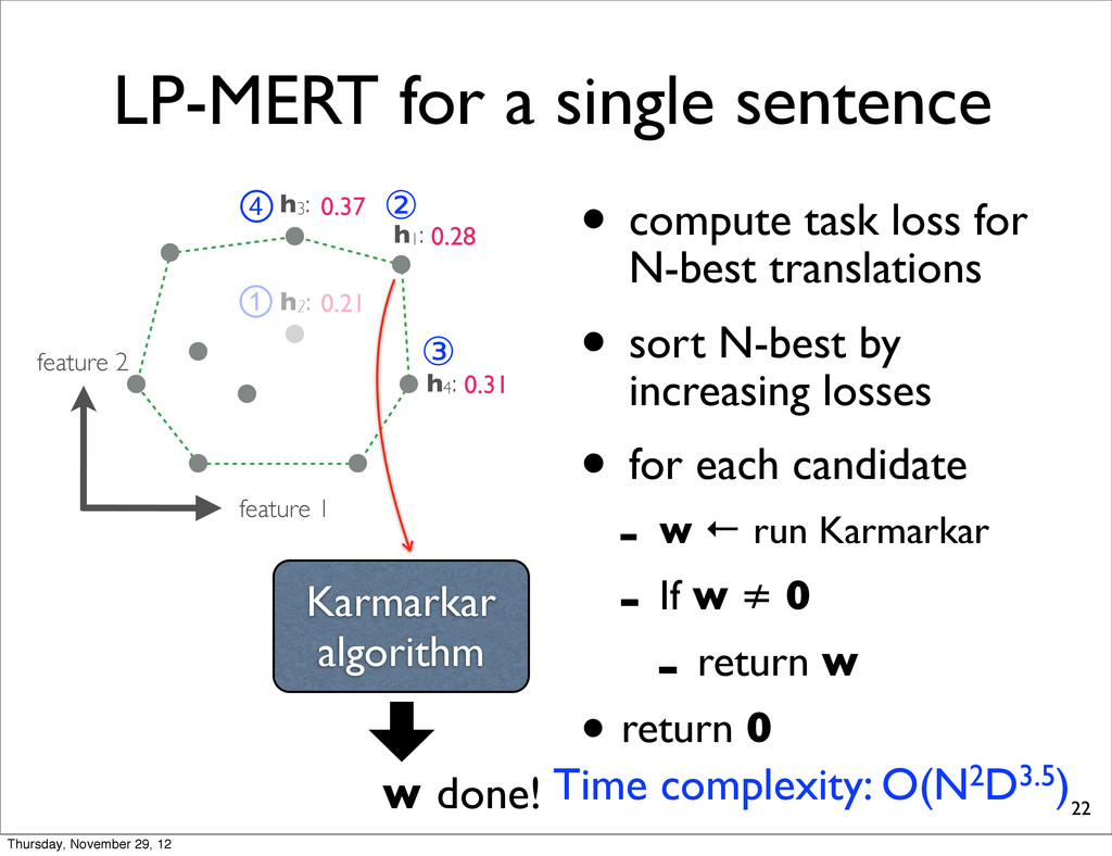
h2: • compute task loss for N-best translations • sort N-best by increasing losses • for each candidate - w ← run Karmarkar - If w ≠ 0 - return w • return 0 h4: h1: h3: 0.28 0.37 0.31 0.21 ① ② ③ ④ Karmarkar algorithm Thursday, November 29, 12
h2: • compute task loss for N-best translations • sort N-best by increasing losses • for each candidate - w ← run Karmarkar - If w ≠ 0 - return w • return 0 h4: h1: h3: 0.28 0.37 0.31 0.21 ① ② ③ ④ Karmarkar algorithm Thursday, November 29, 12
h2: • compute task loss for N-best translations • sort N-best by increasing losses • for each candidate - w ← run Karmarkar - If w ≠ 0 - return w • return 0 h4: h1: h3: 0.28 0.37 0.31 0.21 ① ② ③ ④ Karmarkar algorithm Thursday, November 29, 12
h2: • compute task loss for N-best translations • sort N-best by increasing losses • for each candidate - w ← run Karmarkar - If w ≠ 0 - return w • return 0 h4: h1: h3: 0.28 0.37 0.31 0.21 ① ② ③ ④ Karmarkar algorithm 0 Thursday, November 29, 12
h2: • compute task loss for N-best translations • sort N-best by increasing losses • for each candidate - w ← run Karmarkar - If w ≠ 0 - return w • return 0 h4: h1: h3: 0.28 0.37 0.31 0.21 ① ② ③ ④ Karmarkar algorithm Thursday, November 29, 12
h2: • compute task loss for N-best translations • sort N-best by increasing losses • for each candidate - w ← run Karmarkar - If w ≠ 0 - return w • return 0 h4: h1: h3: 0.28 0.37 0.31 0.21 ① ② ③ ④ Karmarkar algorithm w done! Thursday, November 29, 12
h2: • compute task loss for N-best translations • sort N-best by increasing losses • for each candidate - w ← run Karmarkar - If w ≠ 0 - return w • return 0 h4: h1: h3: 0.28 0.37 0.31 0.21 ① ② ③ ④ Karmarkar algorithm w done! Time complexity: O(N2D3.5) Thursday, November 29, 12
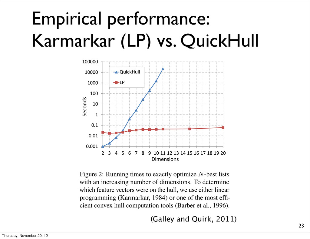
(LP), nonical form c| w Aw b hi in Eq. 3, by defining with an,d = hj,d hi,d ent of hj), and by setting e vertex hi is extreme if nds a non-zero vector w stem. To ensure that w is or, we set c = hi hµ, to be inside the hull (e.g., list).6 In the remaining LP formulation in func- 1 . . . hN ) , which returns izing hi, or which returns h1 . . . hN ) . We also use ote whether hi is extreme 0.001 0.01 0.1 1 10 100 1000 10000 100000 2 3 4 5 6 7 8 9 10 11 12 13 14 15 16 17 18 19 20 QuickHull LP Dimensions Seconds Figure 2: Running times to exactly optimize N-best lists with an increasing number of dimensions. To determine which feature vectors were on the hull, we use either linear programming (Karmarkar, 1984) or one of the most effi- cient convex hull computation tools (Barber et al., 1996). method of (Karmarkar, 1984), and since the main loop may run O ( N ) times in the worst case, time (Galley and Quirk, 2011) Thursday, November 29, 12
(LP), nonical form c| w Aw b hi in Eq. 3, by defining with an,d = hj,d hi,d ent of hj), and by setting e vertex hi is extreme if nds a non-zero vector w stem. To ensure that w is or, we set c = hi hµ, to be inside the hull (e.g., list).6 In the remaining LP formulation in func- 1 . . . hN ) , which returns izing hi, or which returns h1 . . . hN ) . We also use ote whether hi is extreme 0.001 0.01 0.1 1 10 100 1000 10000 100000 2 3 4 5 6 7 8 9 10 11 12 13 14 15 16 17 18 19 20 QuickHull LP Dimensions Seconds Figure 2: Running times to exactly optimize N-best lists with an increasing number of dimensions. To determine which feature vectors were on the hull, we use either linear programming (Karmarkar, 1984) or one of the most effi- cient convex hull computation tools (Barber et al., 1996). method of (Karmarkar, 1984), and since the main loop may run O ( N ) times in the worst case, time (Galley and Quirk, 2011) O(ND3.5) O(NbD/2c+1) Thursday, November 29, 12
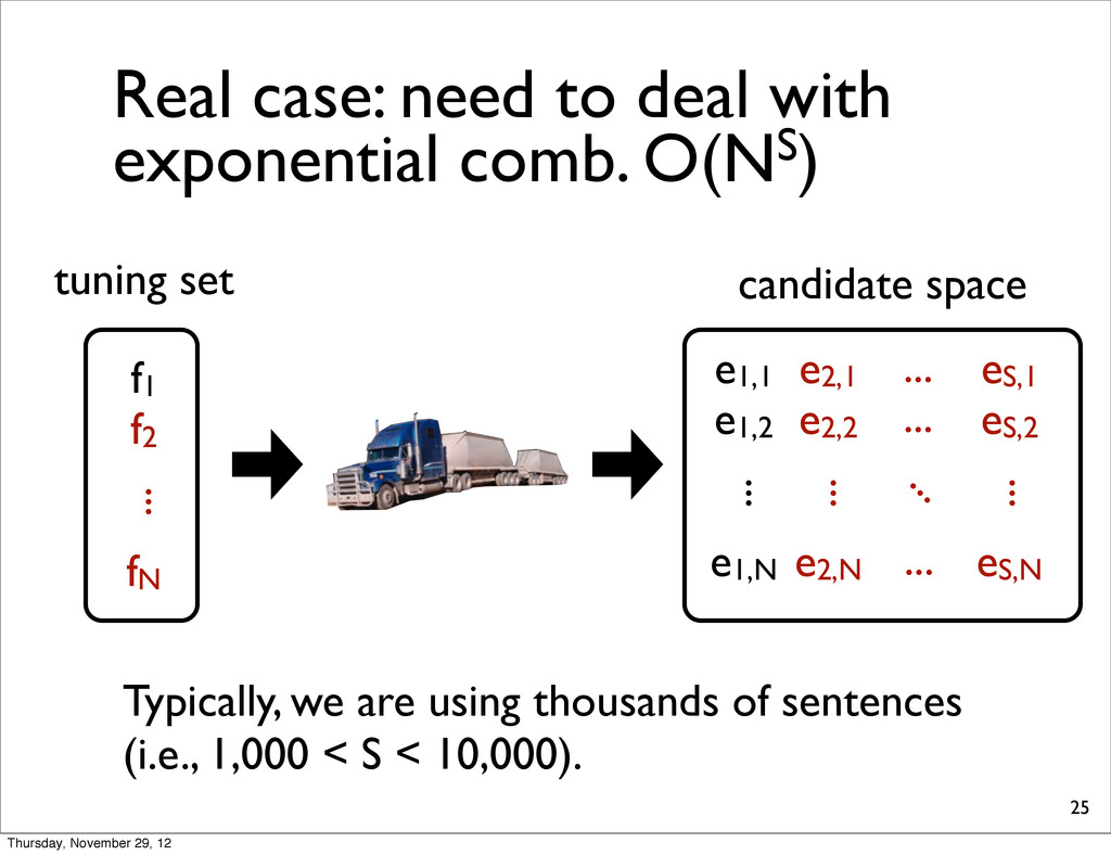
tuning set f1 f2 fN ... candidate space e1,1 e1,2 e1,N ... e2,1 e2,2 e2,N ... eS,1 eS,2 eS,N ... ... ... ... ... Typically, we are using thousands of sentences (i.e., 1,000 < S < 10,000). Thursday, November 29, 12
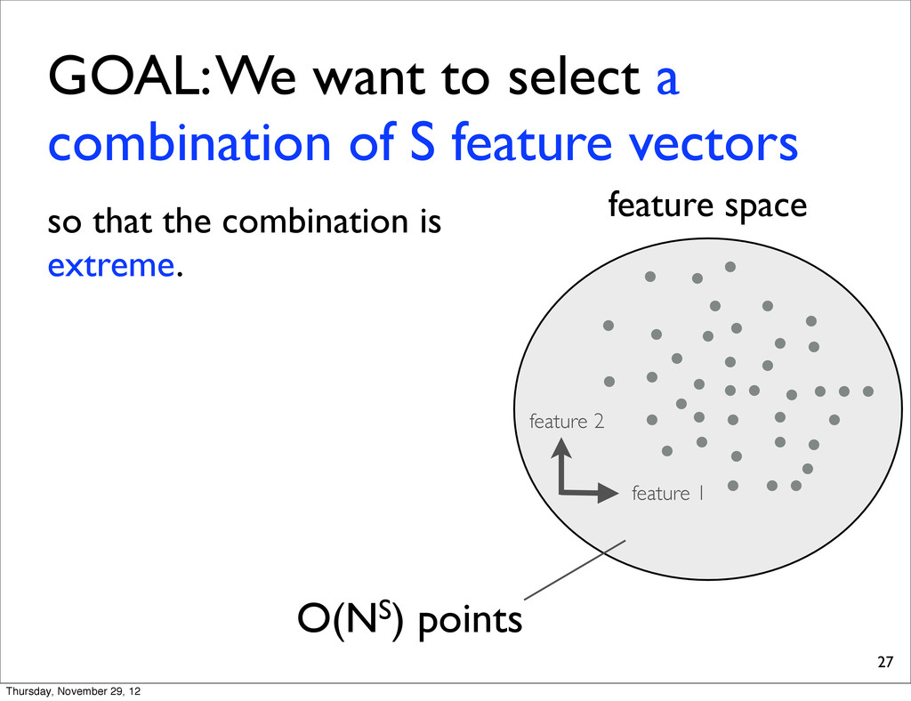
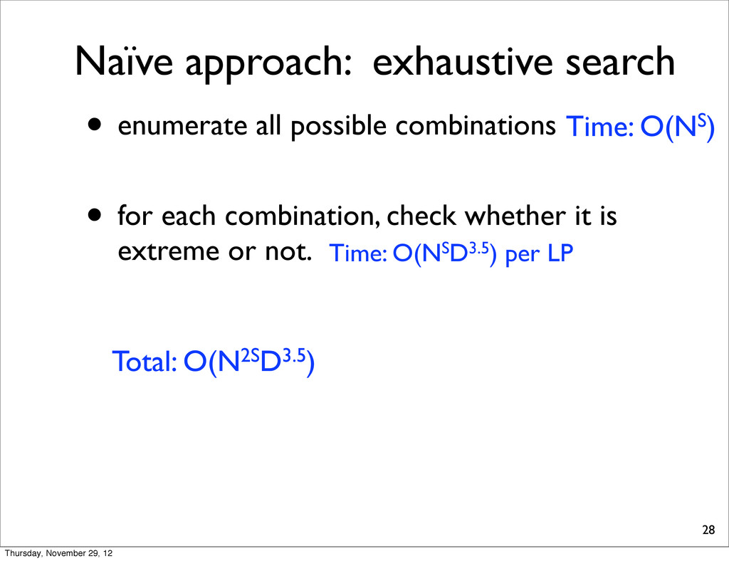
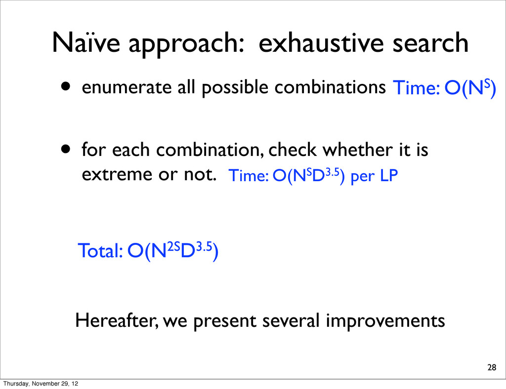
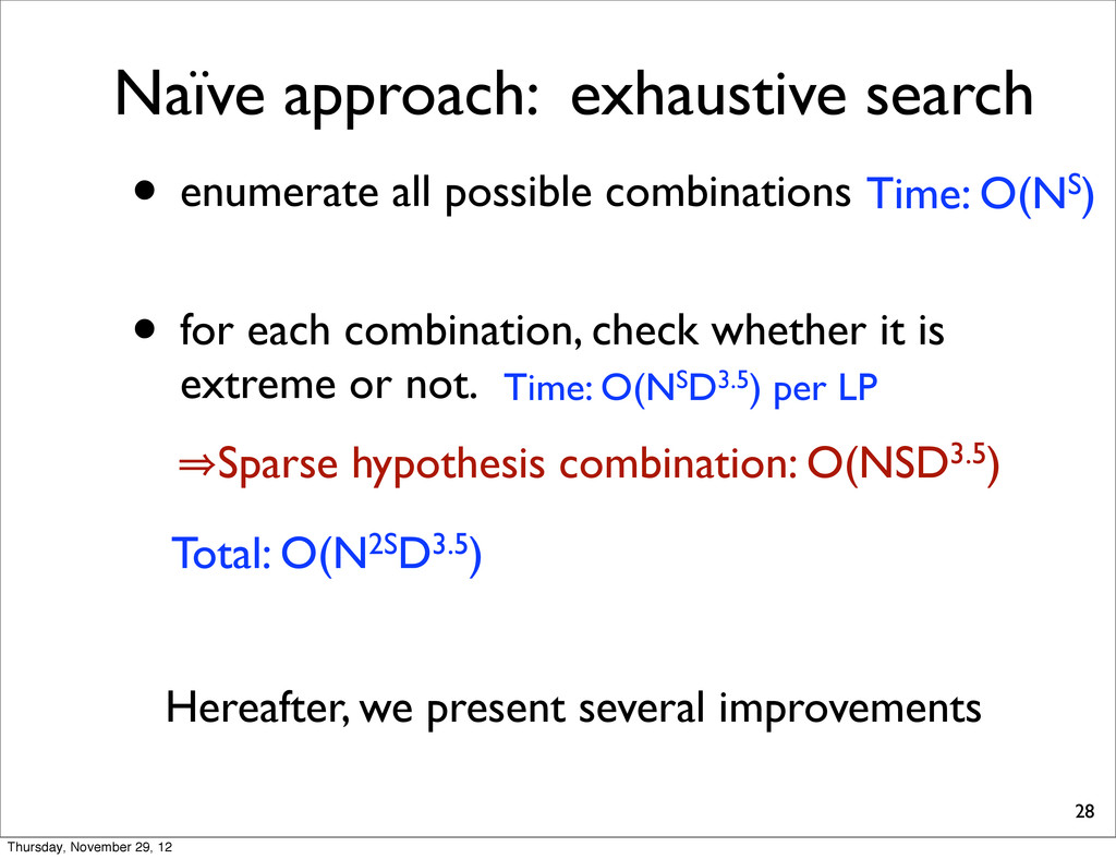
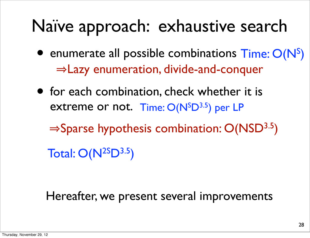
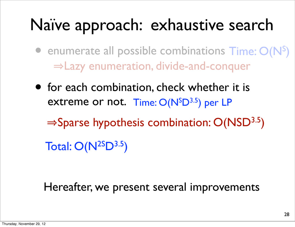
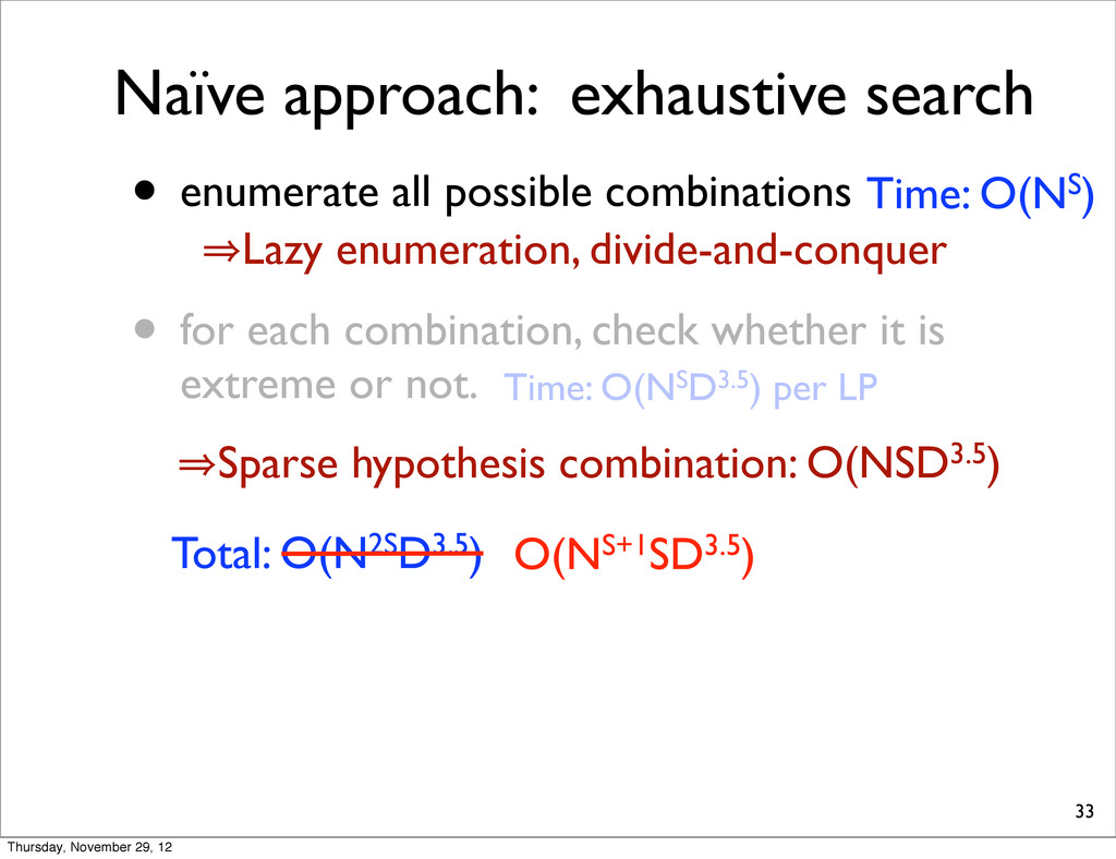
for each combination, check whether it is extreme or not. 28 Time: O(NSD3.5) per LP Total: O(N2SD3.5) Hereafter, we present several improvements Time: O(NS) Thursday, November 29, 12
for each combination, check whether it is extreme or not. 28 Time: O(NSD3.5) per LP Total: O(N2SD3.5) Hereafter, we present several improvements Time: O(NS) 㱺Sparse hypothesis combination: O(NSD3.5) Thursday, November 29, 12
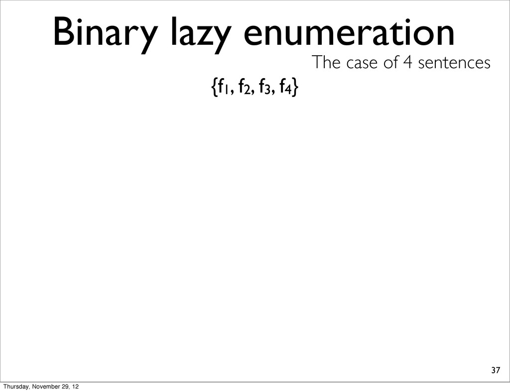
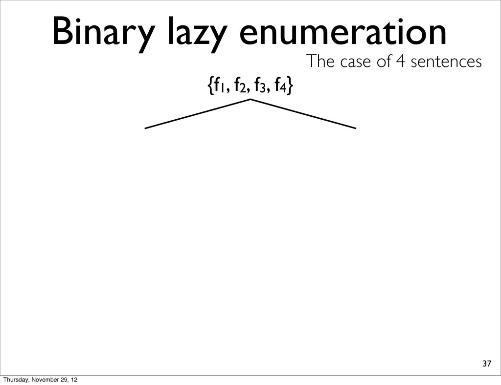
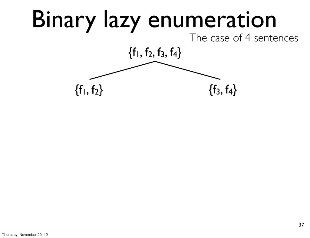
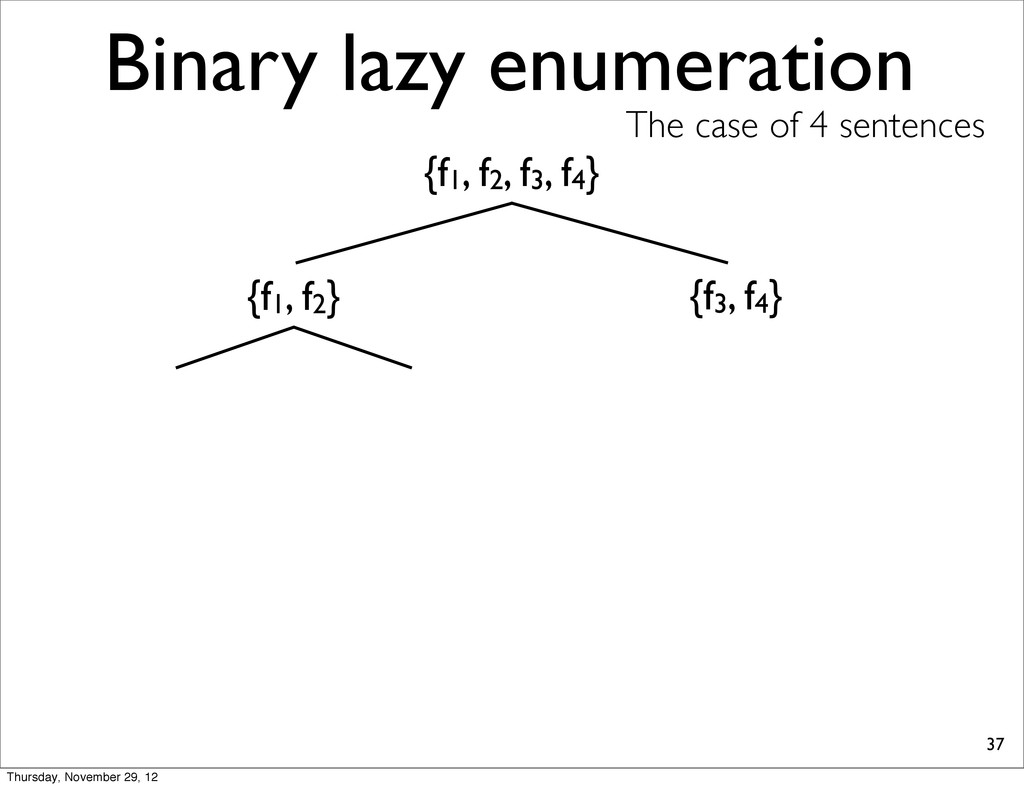
for each combination, check whether it is extreme or not. 28 Time: O(NSD3.5) per LP Total: O(N2SD3.5) Hereafter, we present several improvements Time: O(NS) 㱺Sparse hypothesis combination: O(NSD3.5) 㱺Lazy enumeration, divide-and-conquer Thursday, November 29, 12
for each combination, check whether it is extreme or not. 28 Time: O(NSD3.5) per LP Total: O(N2SD3.5) Hereafter, we present several improvements Time: O(NS) 㱺Sparse hypothesis combination: O(NSD3.5) 㱺Lazy enumeration, divide-and-conquer Thursday, November 29, 12
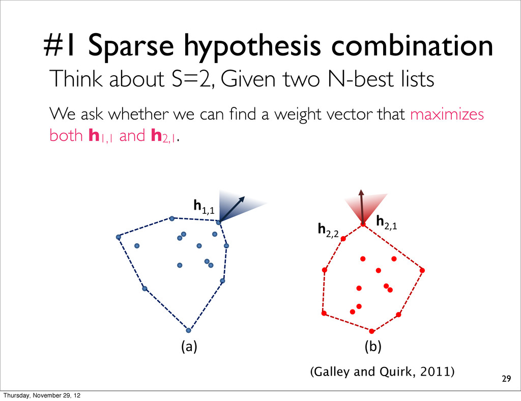
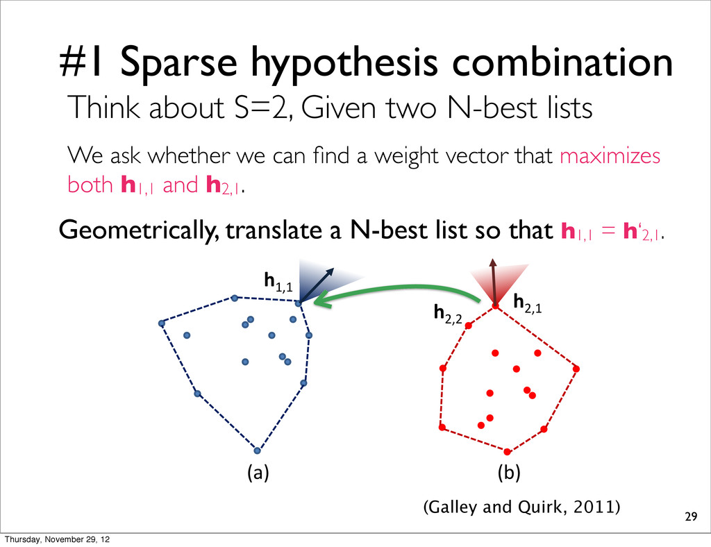
nd return loss. It is it follows low since whether ST ) time h1,1 h2,2 h2,1 (a) (b) (Galley and Quirk, 2011) Think about S=2, Given two N-best lists We ask whether we can find a weight vector that maximizes both h1,1 and h2,1. Thursday, November 29, 12
nd return loss. It is it follows low since whether ST ) time h1,1 h2,2 h2,1 (a) (b) (Galley and Quirk, 2011) Think about S=2, Given two N-best lists We ask whether we can find a weight vector that maximizes both h1,1 and h2,1. Geometrically, translate a N-best list so that h1,1 = h‘2,1. Thursday, November 29, 12
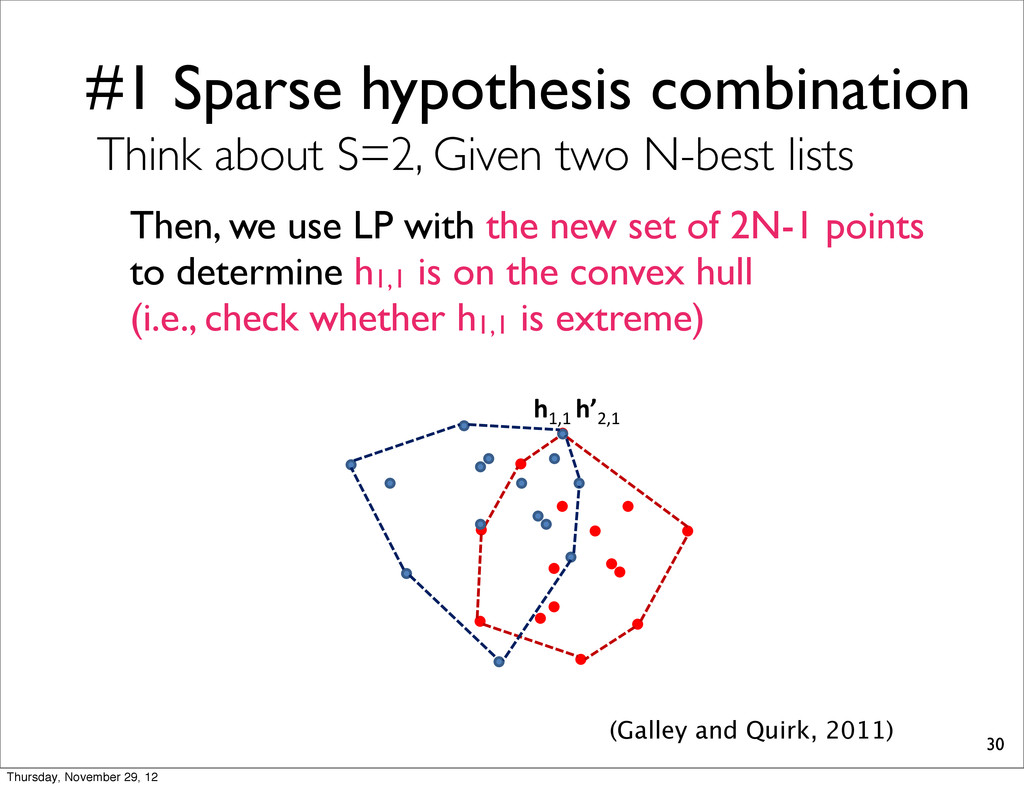
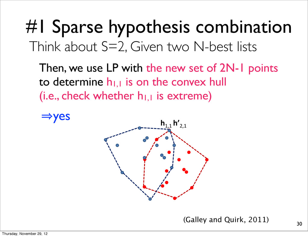
about S=2, Given two N-best lists Then, we use LP with the new set of 2N-1 points to determine h1,1 is on the convex hull (i.e., check whether h1,1 is extreme) s this optimization sible combinations determine for each extreme, and return west total loss. It is mal (since it follows ibitively slow since determine whether ires O ( NST ) time ) time in total. We nts to make this ap- ination ed above, each LP h [ m ]; H ) requires s NS vertices, but (c) h1,1 h’2,1 Thursday, November 29, 12
about S=2, Given two N-best lists Then, we use LP with the new set of 2N-1 points to determine h1,1 is on the convex hull (i.e., check whether h1,1 is extreme) s this optimization sible combinations determine for each extreme, and return west total loss. It is mal (since it follows ibitively slow since determine whether ires O ( NST ) time ) time in total. We nts to make this ap- ination ed above, each LP h [ m ]; H ) requires s NS vertices, but (c) h1,1 h’2,1 㱺yes Thursday, November 29, 12
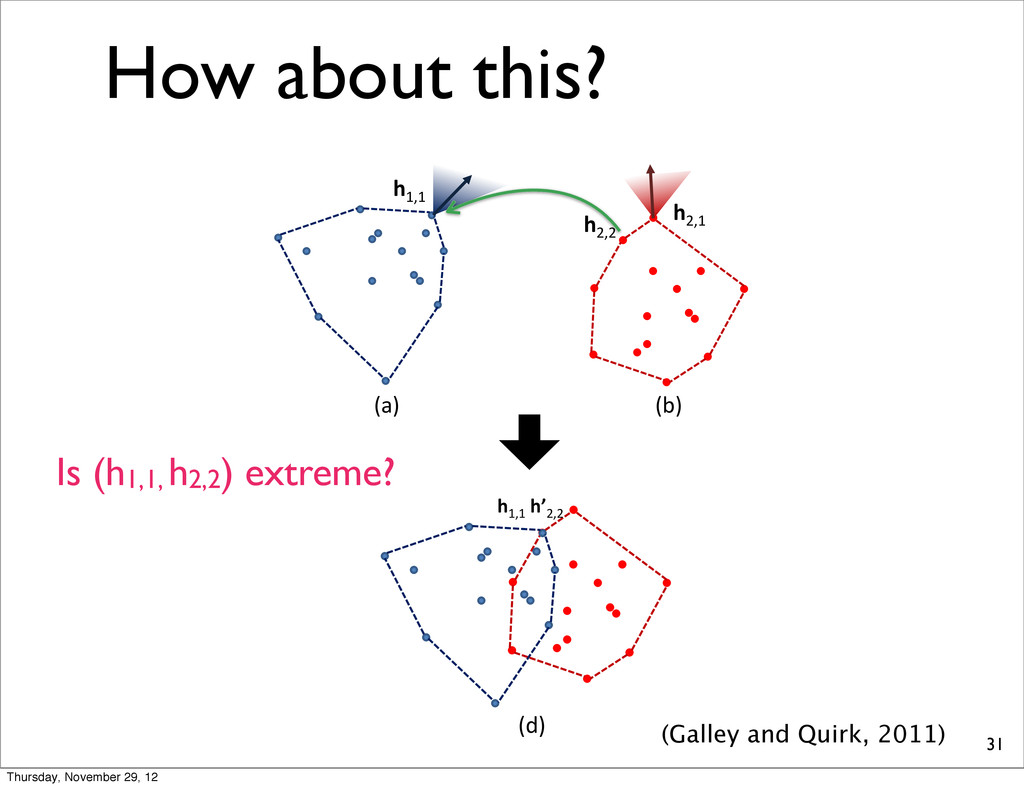
each xtreme, and return est total loss. It is al (since it follows bitively slow since etermine whether res O ( NST ) time ) time in total. We s to make this ap- nation d above, each LP [ m ]; H ) requires NS vertices, but o O ( NST ) time. h1,1 h2,2 h2,1 (a) (b) Figure 3: Given two N-best lists, (a) and (b), we use linear programming to determine which hypothesis com- ation ions each eturn It is lows ince ether time . We s ap- h LP uires h1,1 h’2,2 (d) (Galley and Quirk, 2011) Is (h1,1, h2,2) extreme? Thursday, November 29, 12
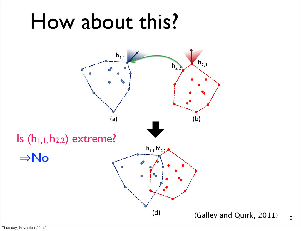
each xtreme, and return est total loss. It is al (since it follows bitively slow since etermine whether res O ( NST ) time ) time in total. We s to make this ap- nation d above, each LP [ m ]; H ) requires NS vertices, but o O ( NST ) time. h1,1 h2,2 h2,1 (a) (b) Figure 3: Given two N-best lists, (a) and (b), we use linear programming to determine which hypothesis com- ation ions each eturn It is lows ince ether time . We s ap- h LP uires h1,1 h’2,2 (d) (Galley and Quirk, 2011) Is (h1,1, h2,2) extreme? 㱺No Thursday, November 29, 12
S(N-1) + 1 points instead of NS to determine whether a given point is extreme. • This trick does not sacrifice the optimality of LP-MERT. See appendix for details. 32 Thursday, November 29, 12
for each combination, check whether it is extreme or not. 33 Time: O(NSD3.5) per LP Total: O(N2SD3.5) Time: O(NS) 㱺Sparse hypothesis combination: O(NSD3.5) 㱺Lazy enumeration, divide-and-conquer O(NS+1SD3.5) Thursday, November 29, 12
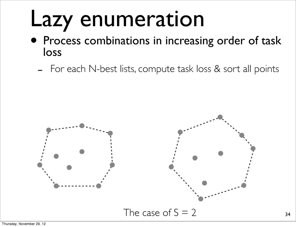
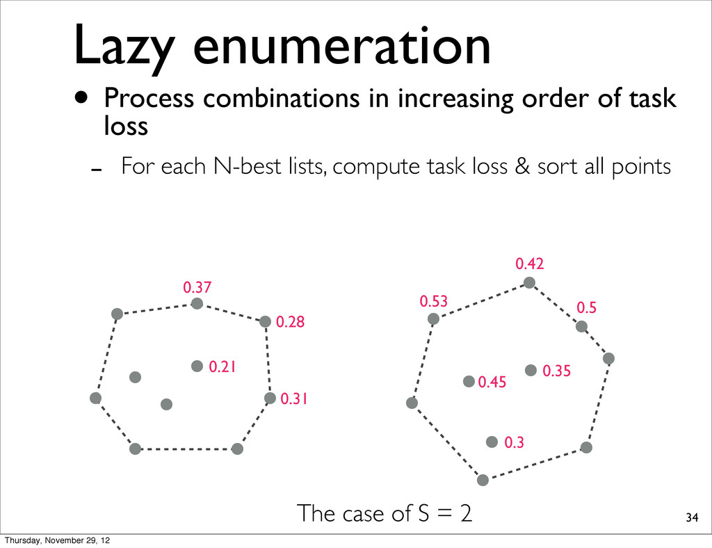
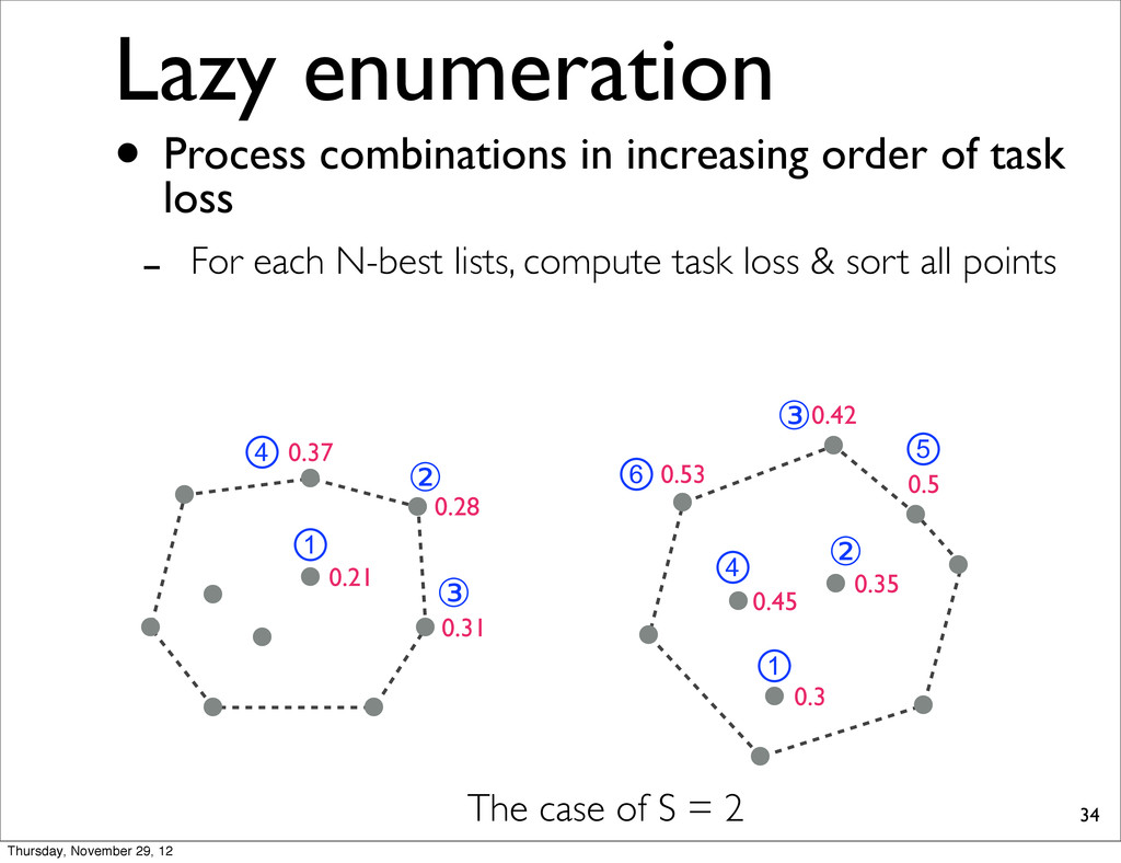
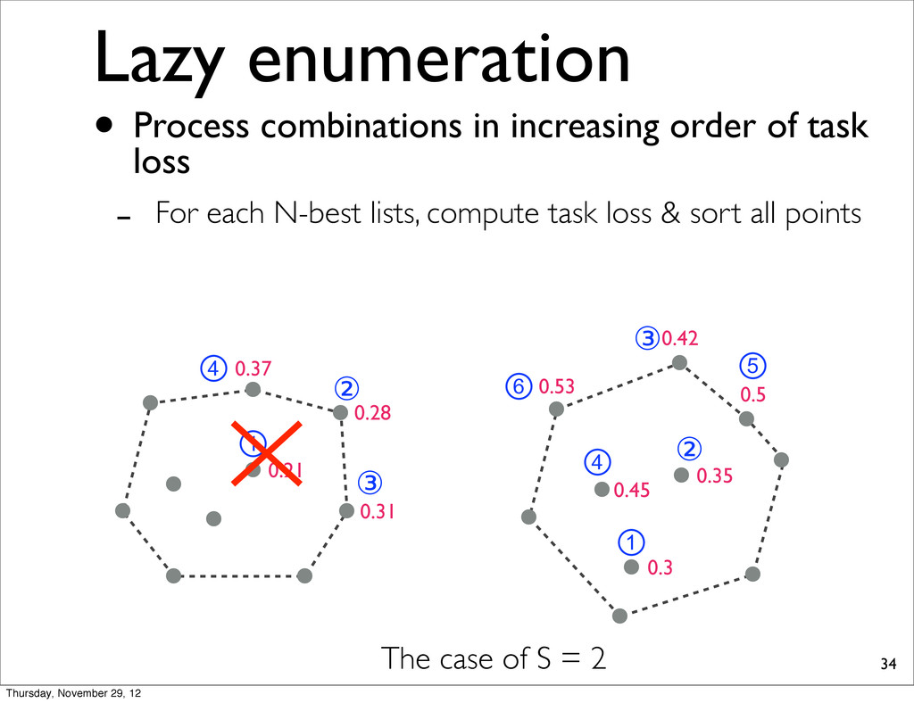
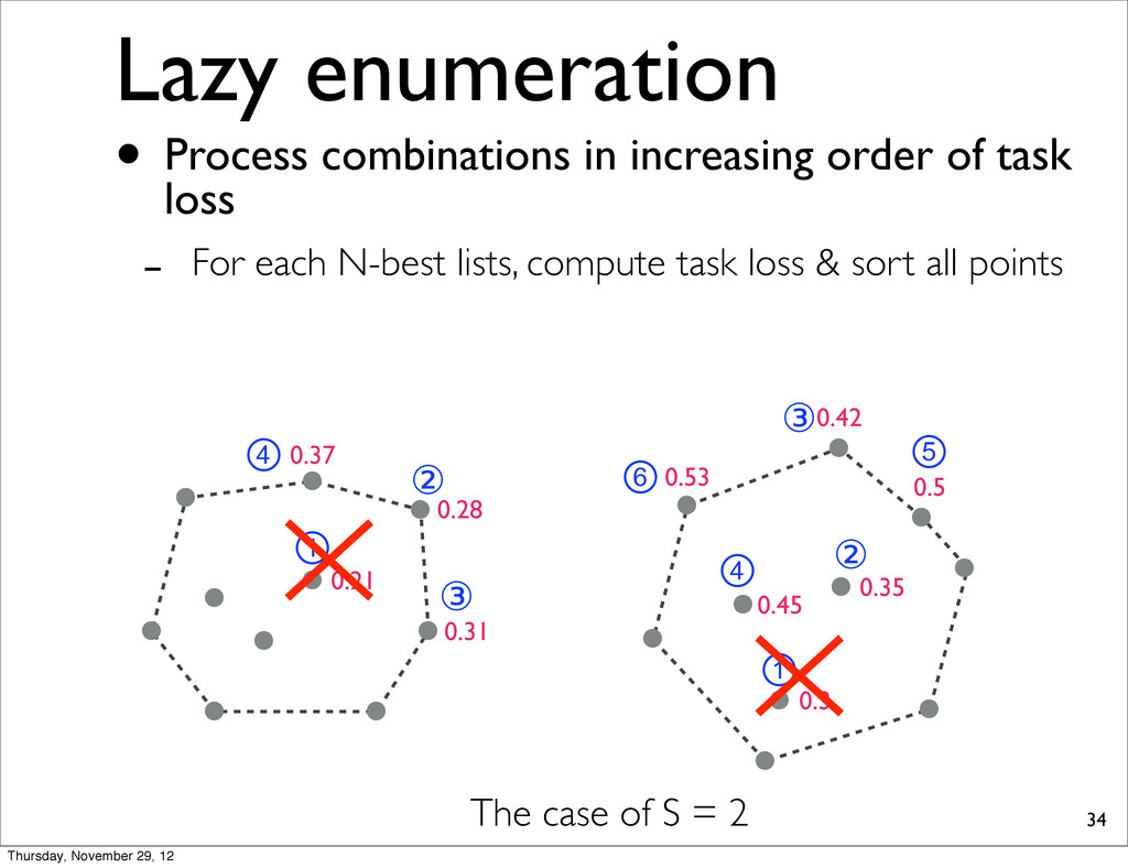
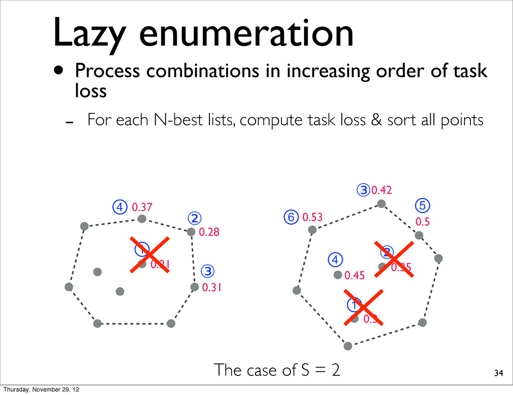
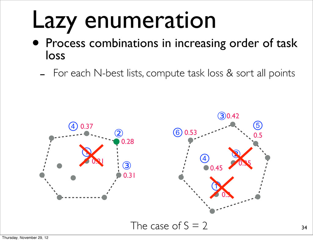
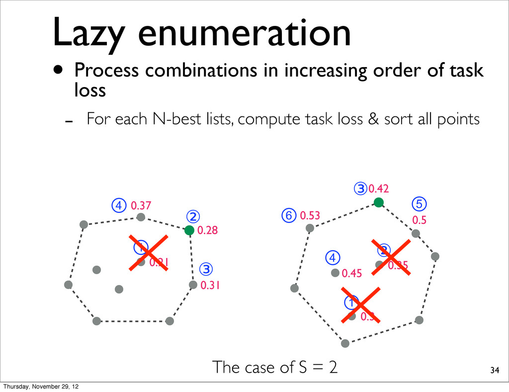
0.37 0.31 0.21 The case of S = 2 • Process combinations in increasing order of task loss - For each N-best lists, compute task loss & sort all points Thursday, November 29, 12
0.37 0.31 0.21 ① ② ③ ④ ⑥ ① ② ③ ④ ⑤ The case of S = 2 • Process combinations in increasing order of task loss - For each N-best lists, compute task loss & sort all points Thursday, November 29, 12
0.37 0.31 0.21 ① ② ③ ④ ⑥ ① ② ③ ④ ⑤ The case of S = 2 • Process combinations in increasing order of task loss - For each N-best lists, compute task loss & sort all points Thursday, November 29, 12
0.37 0.31 0.21 ① ② ③ ④ ⑥ ① ② ③ ④ ⑤ The case of S = 2 • Process combinations in increasing order of task loss - For each N-best lists, compute task loss & sort all points Thursday, November 29, 12
0.37 0.31 0.21 ① ② ③ ④ ⑥ ① ② ③ ④ ⑤ The case of S = 2 • Process combinations in increasing order of task loss - For each N-best lists, compute task loss & sort all points Thursday, November 29, 12
0.37 0.31 0.21 ① ② ③ ④ ⑥ ① ② ③ ④ ⑤ The case of S = 2 • Process combinations in increasing order of task loss - For each N-best lists, compute task loss & sort all points Thursday, November 29, 12
0.37 0.31 0.21 ① ② ③ ④ ⑥ ① ② ③ ④ ⑤ The case of S = 2 • Process combinations in increasing order of task loss - For each N-best lists, compute task loss & sort all points Thursday, November 29, 12
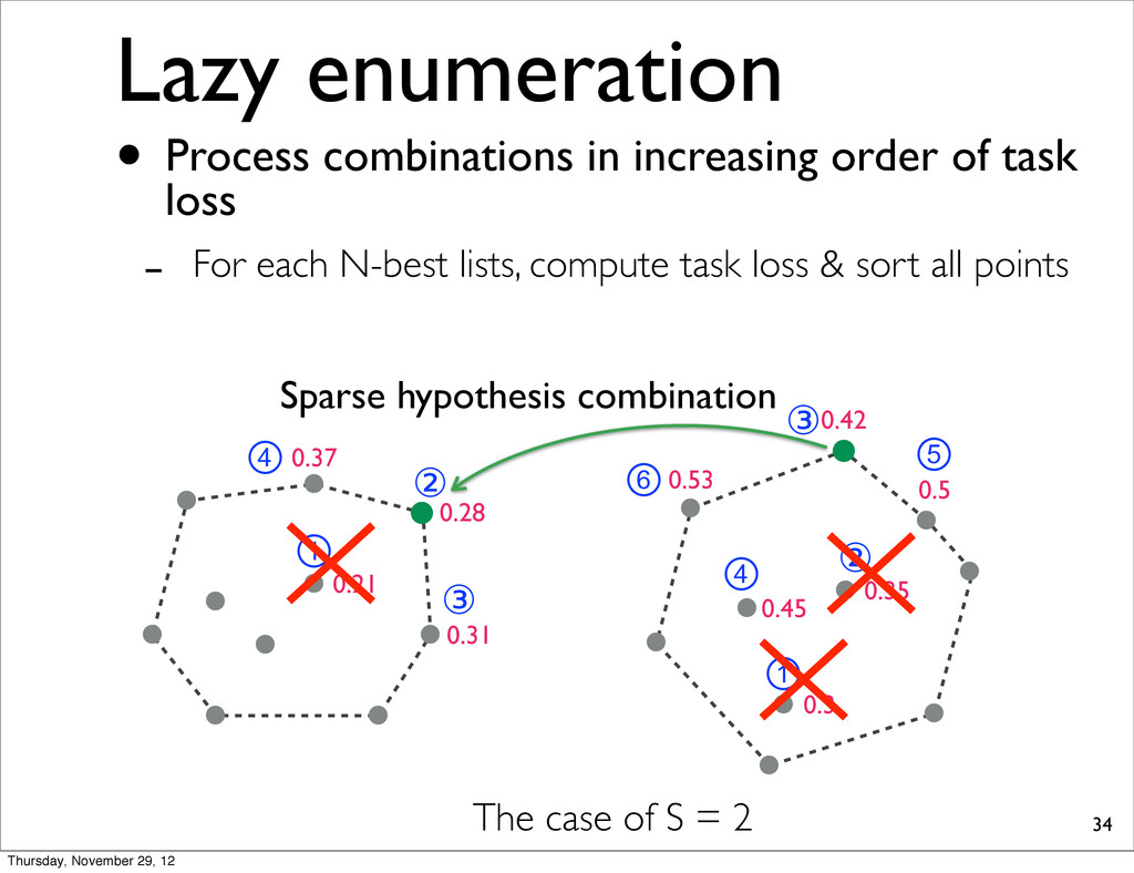
0.37 0.31 0.21 ① ② ③ ④ ⑥ ① ② ③ ④ ⑤ The case of S = 2 Sparse hypothesis combination • Process combinations in increasing order of task loss - For each N-best lists, compute task loss & sort all points Thursday, November 29, 12
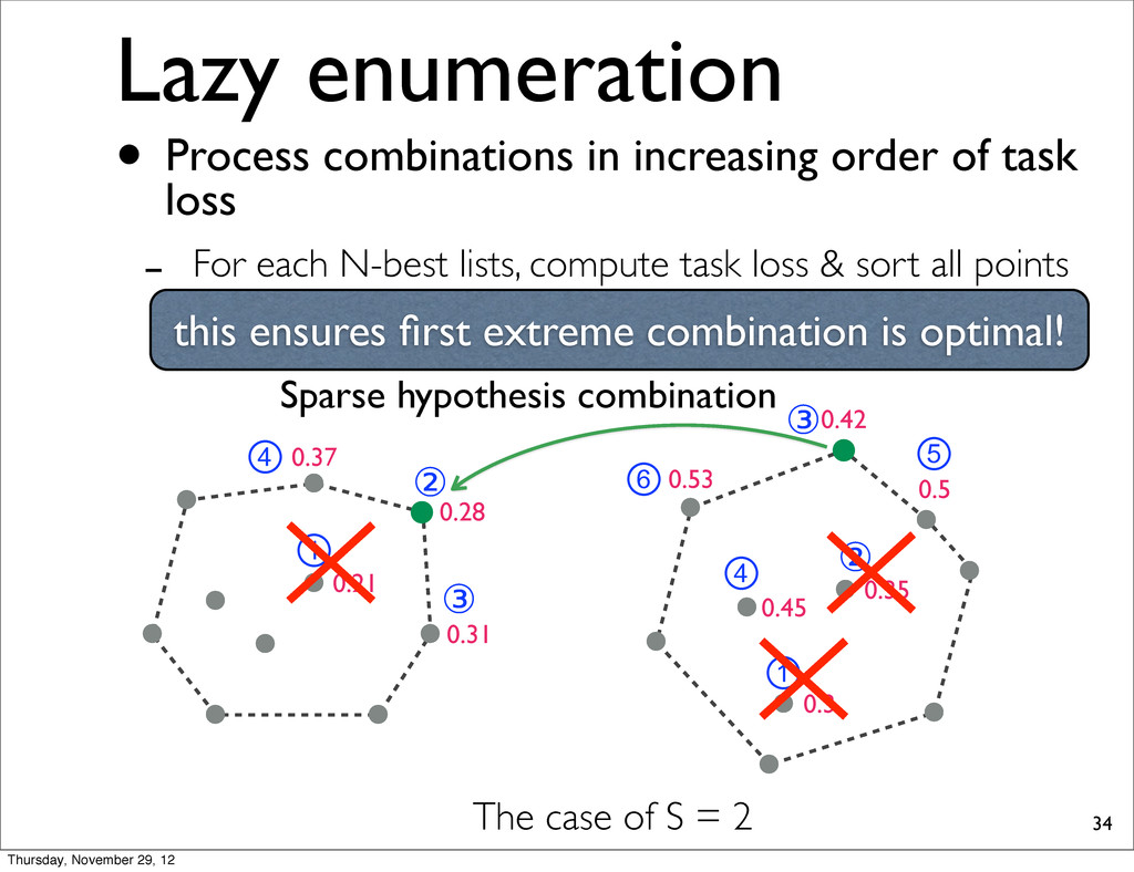
0.37 0.31 0.21 ① ② ③ ④ ⑥ ① ② ③ ④ ⑤ The case of S = 2 Sparse hypothesis combination this ensures first extreme combination is optimal! • Process combinations in increasing order of task loss - For each N-best lists, compute task loss & sort all points Thursday, November 29, 12
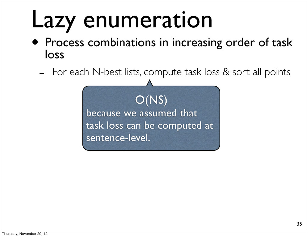
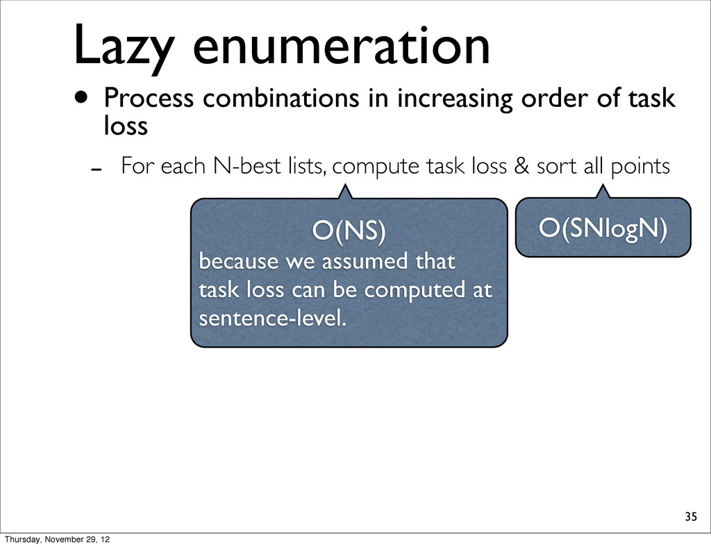
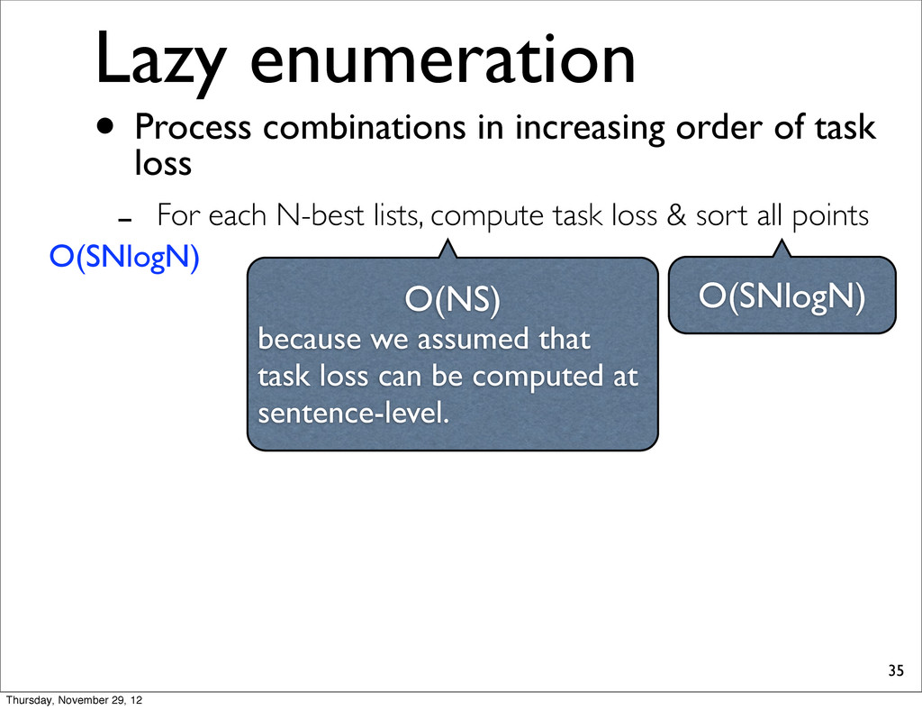
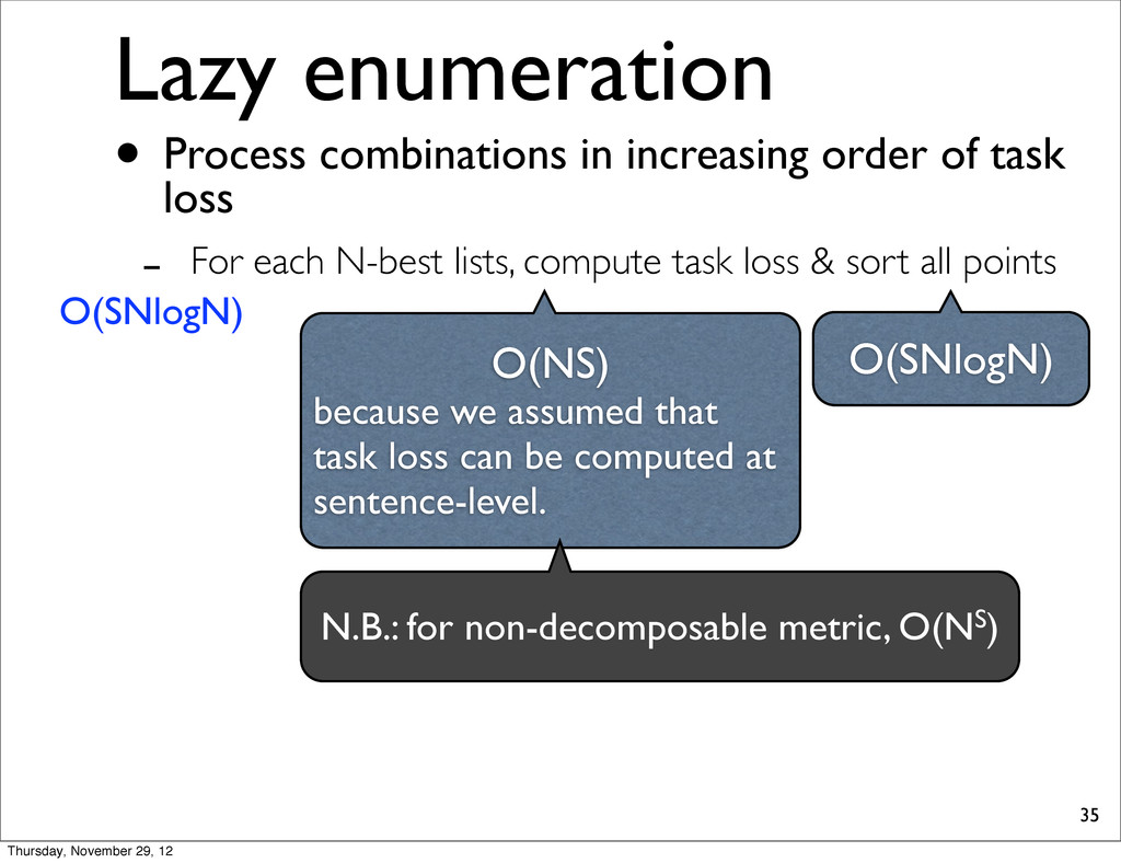
computed at sentence-level. Lazy enumeration • Process combinations in increasing order of task loss - For each N-best lists, compute task loss & sort all points Thursday, November 29, 12
computed at sentence-level. O(SNlogN) Lazy enumeration • Process combinations in increasing order of task loss - For each N-best lists, compute task loss & sort all points Thursday, November 29, 12
be computed at sentence-level. O(SNlogN) Lazy enumeration • Process combinations in increasing order of task loss - For each N-best lists, compute task loss & sort all points Thursday, November 29, 12
be computed at sentence-level. O(SNlogN) N.B.: for non-decomposable metric, O(NS) Lazy enumeration • Process combinations in increasing order of task loss - For each N-best lists, compute task loss & sort all points Thursday, November 29, 12
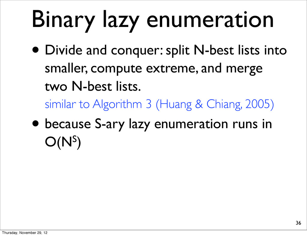
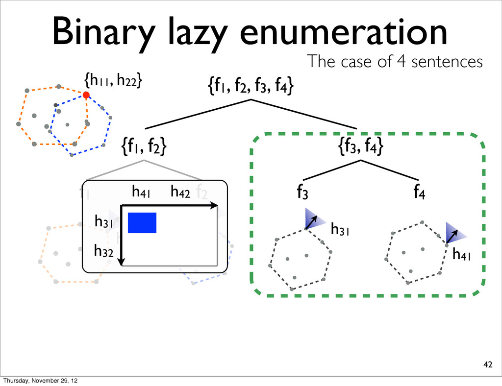
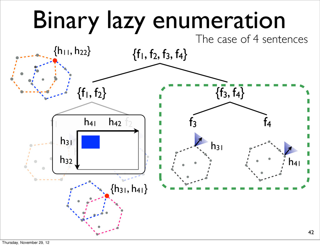
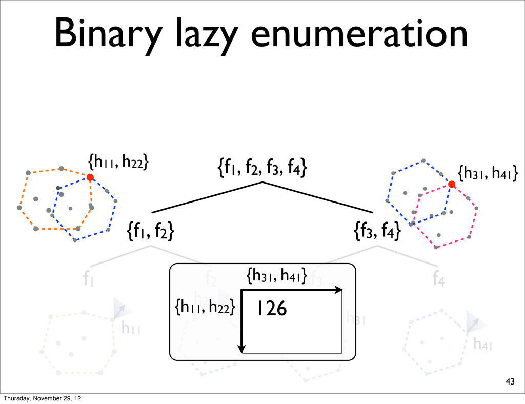
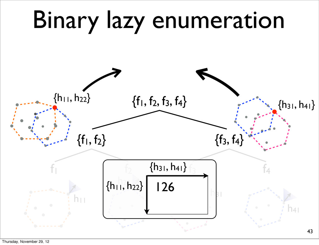
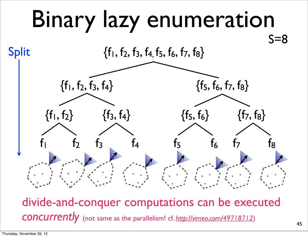
lists into smaller, compute extreme, and merge two N-best lists. • because S-ary lazy enumeration runs in O(NS) similar to Algorithm 3 (Huang & Chiang, 2005) Thursday, November 29, 12
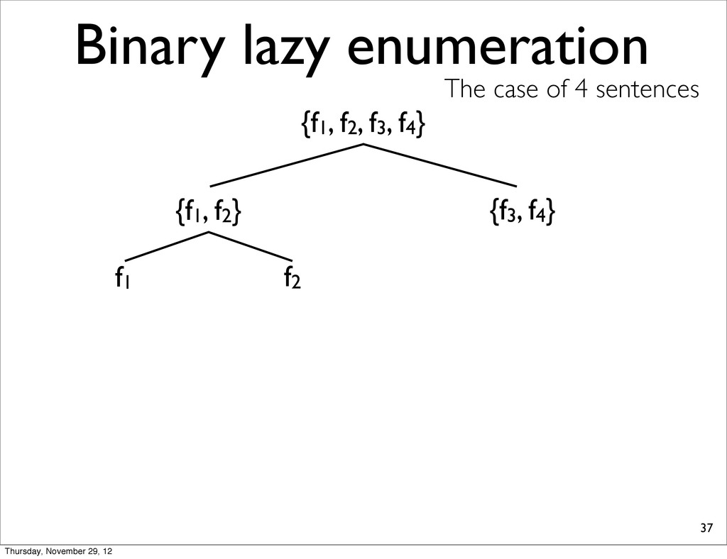
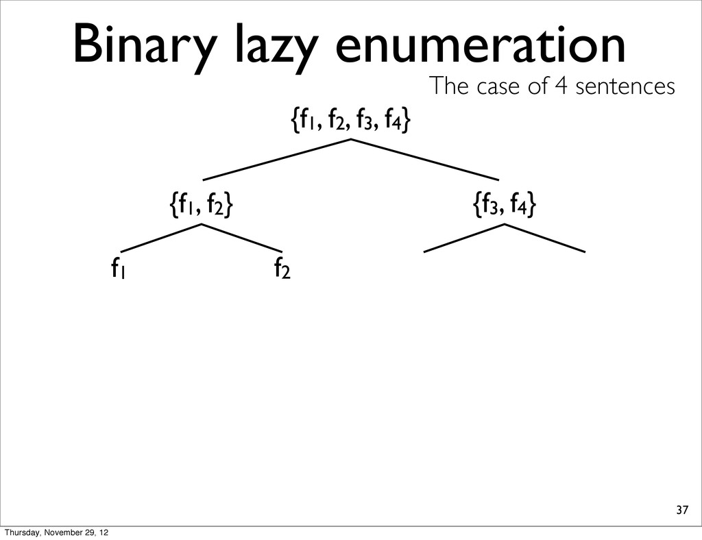
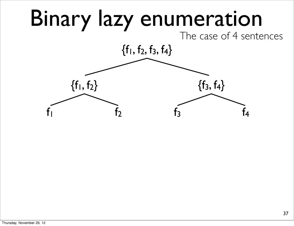
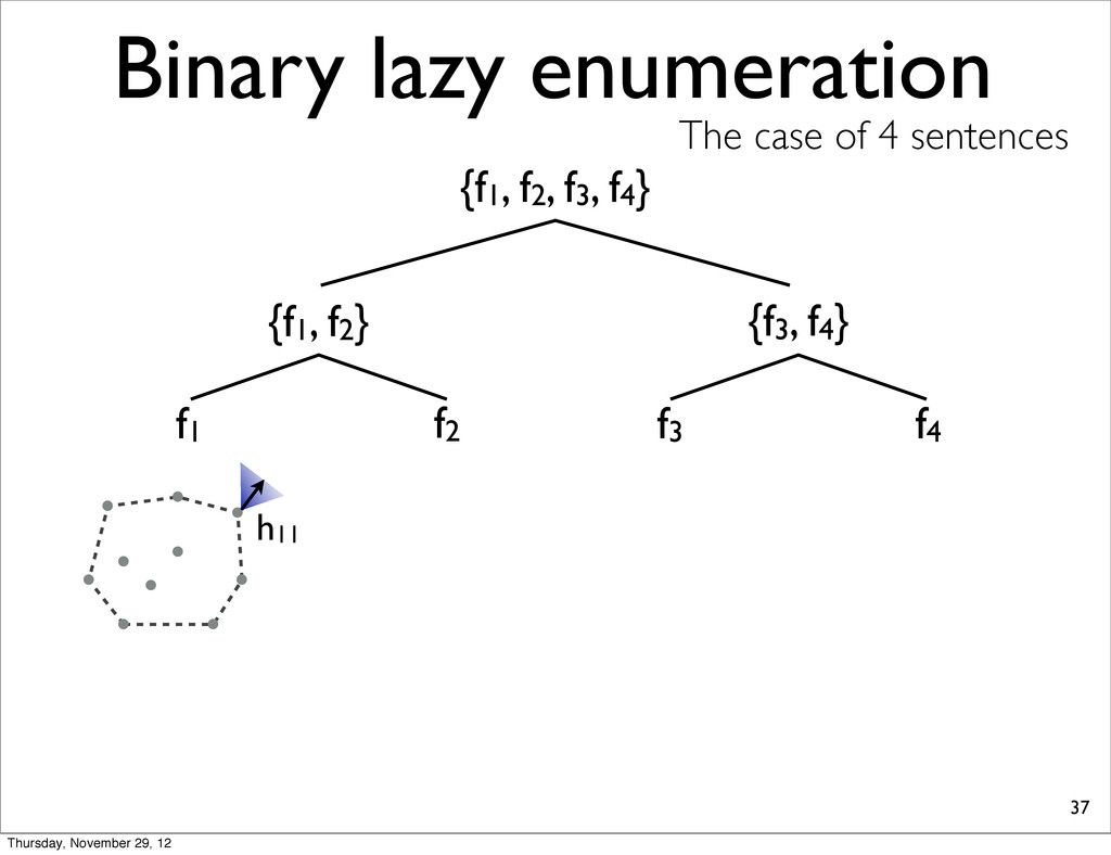
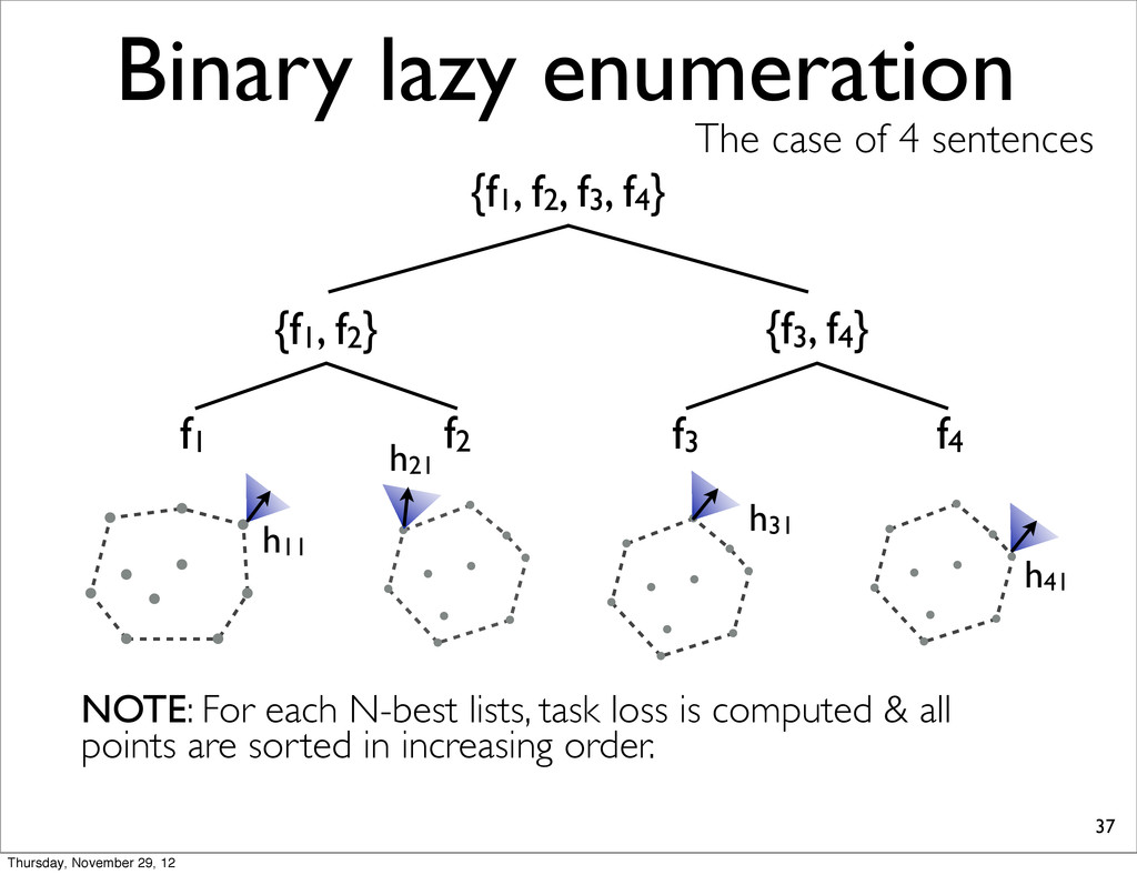
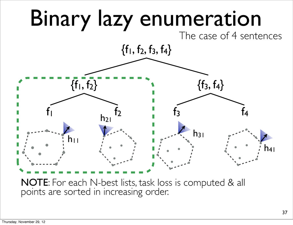
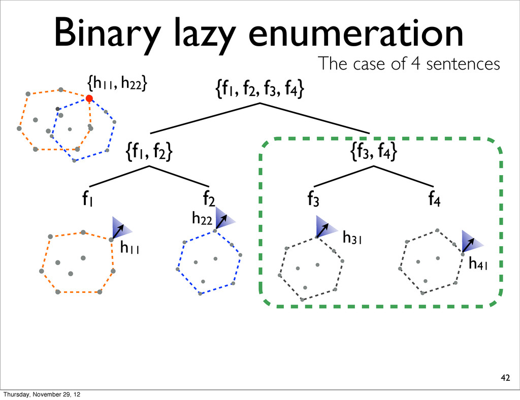
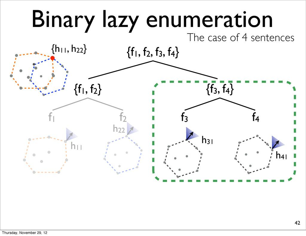
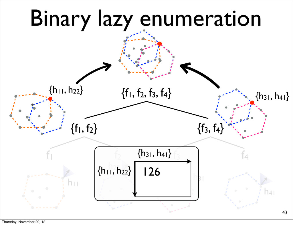
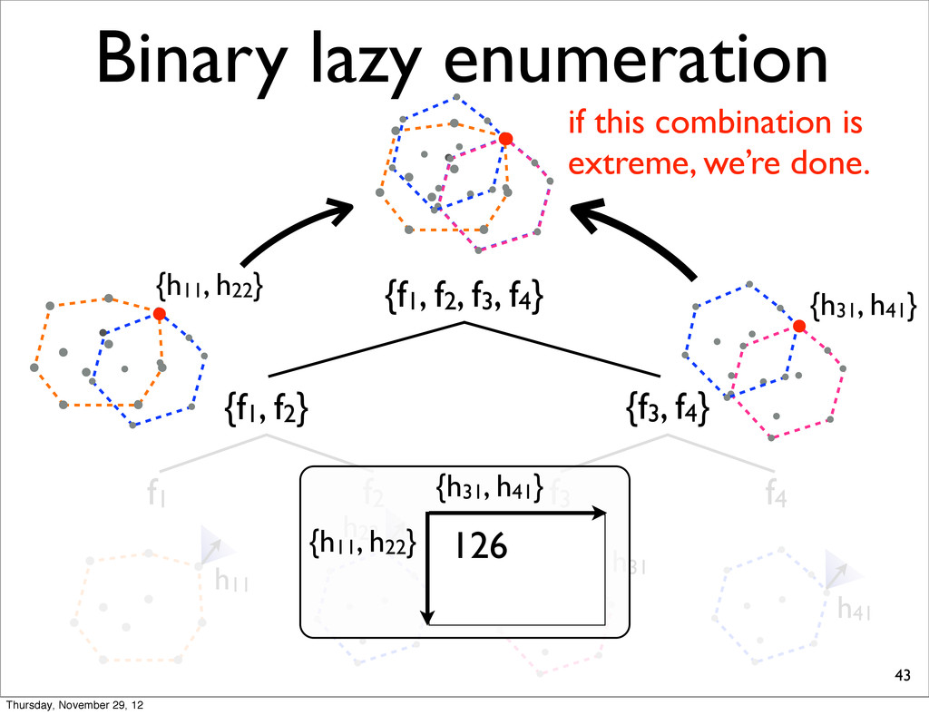
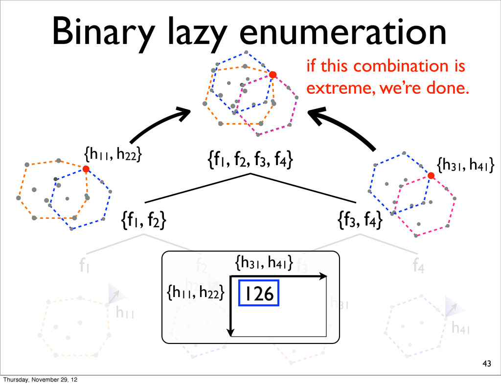
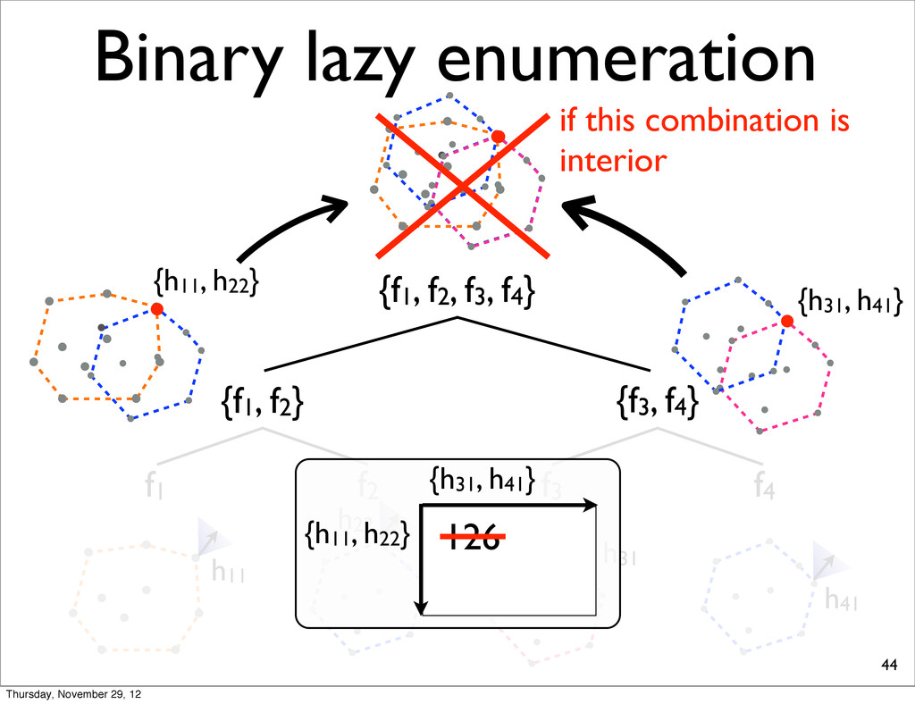
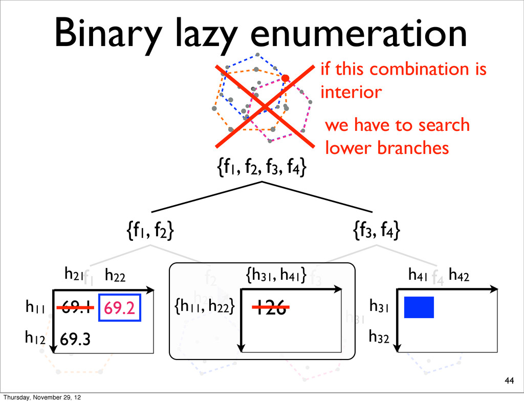
f2, f3, f4} {f1, f2} {f3, f4} f1 f2 f3 f4 h11 NOTE: For each N-best lists, task loss is computed & all points are sorted in increasing order. h31 h41 h21 Thursday, November 29, 12
f2, f3, f4} {f1, f2} {f3, f4} f1 f2 f3 f4 h11 NOTE: For each N-best lists, task loss is computed & all points are sorted in increasing order. h31 h41 h21 Thursday, November 29, 12
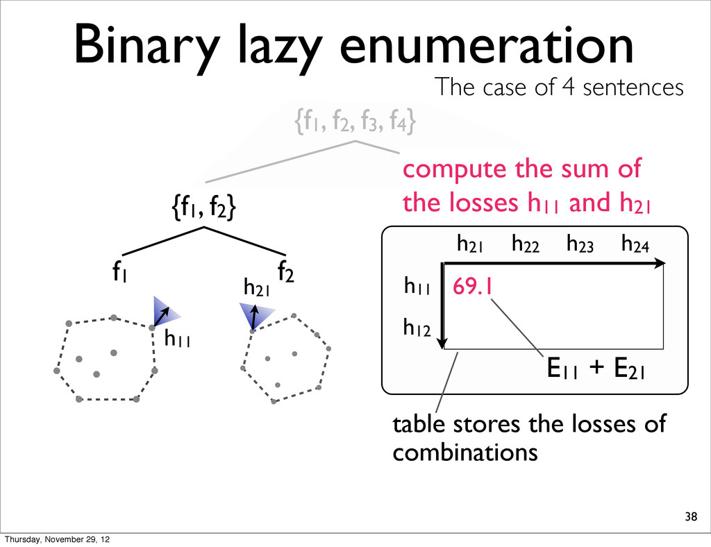
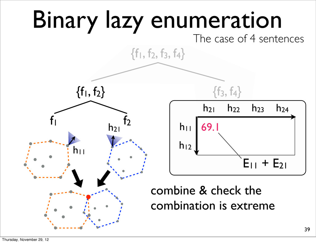
The case of 4 sentences {f1, f2} f1 f2 h11 table stores the losses of combinations h11 h21 69.1 E11 + E21 compute the sum of the losses h11 and h21 h21 h22 h12 h23 h24 Thursday, November 29, 12
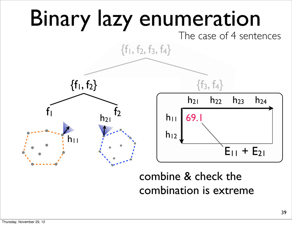
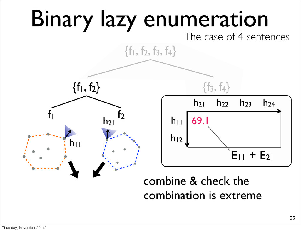
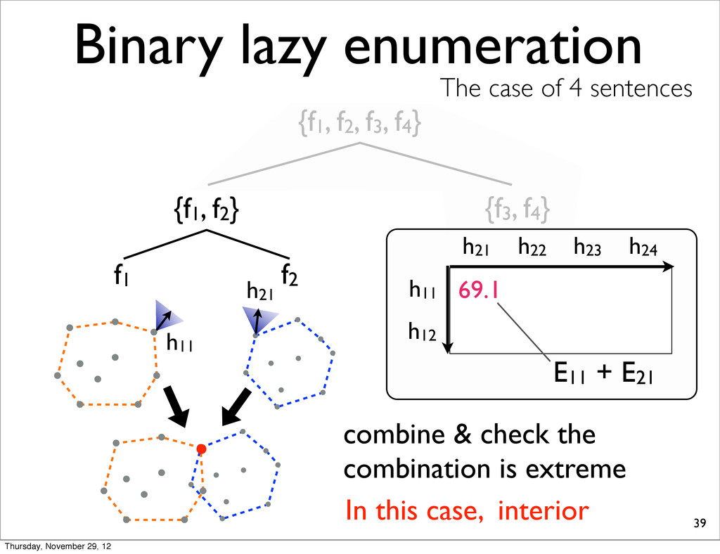
The case of 4 sentences {f1, f2} f1 f2 h11 h21 h11 69.1 E11 + E21 combine & check the combination is extreme In this case, interior h12 h23 h24 h21 h11 h21 69.1 E11 + E21 h22 Thursday, November 29, 12
The case of 4 sentences {f1, f2} f1 f2 h11 h21 h11 69.1 E11 + E21 combine & check the combination is extreme In this case, interior h12 h23 h24 h21 h11 h21 69.1 E11 + E21 h22 Thursday, November 29, 12
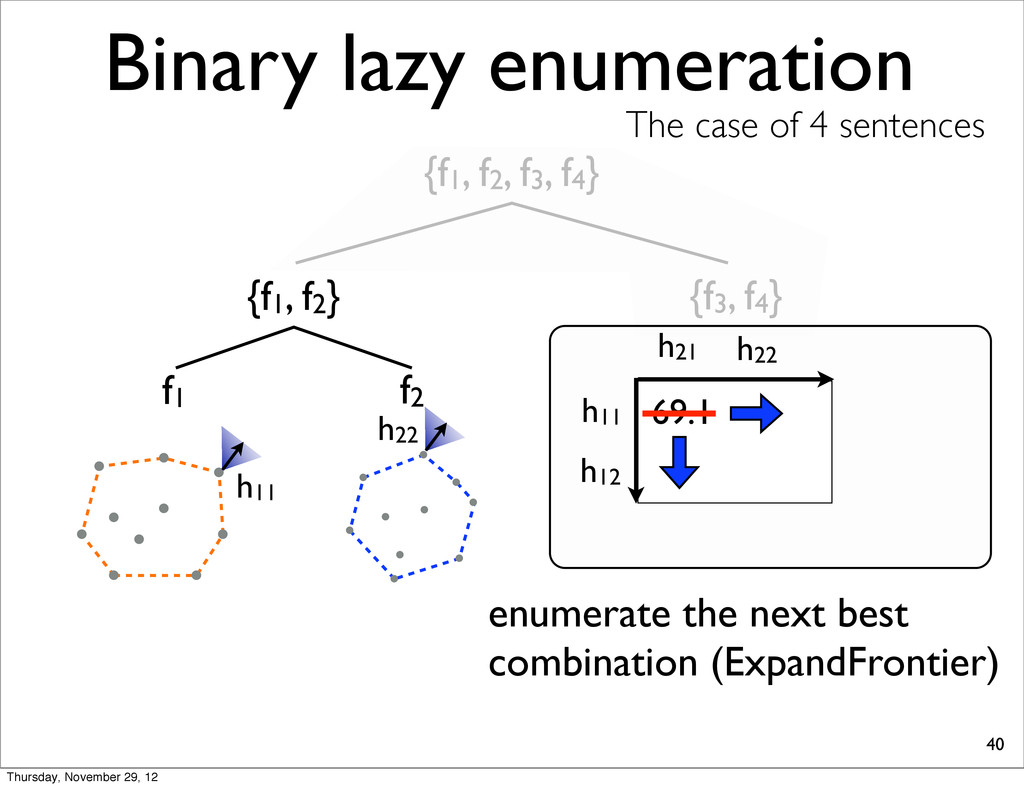
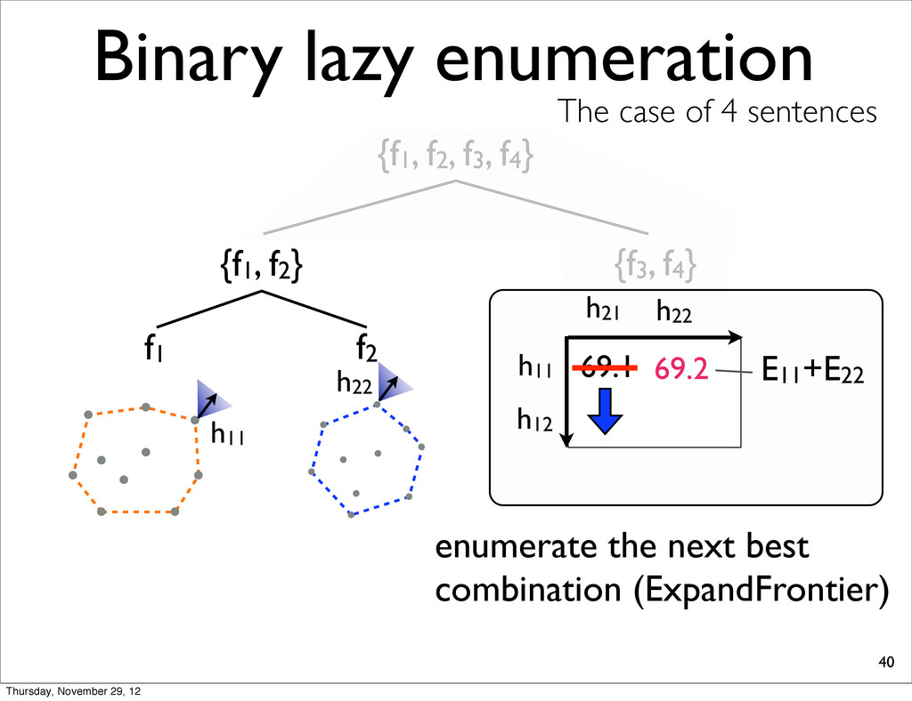
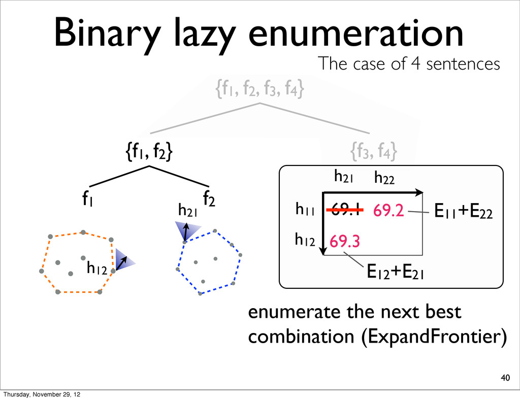
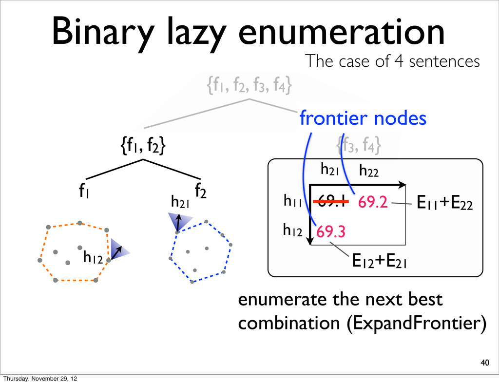
The case of 4 sentences {f1, f2} f1 f2 h11 h11 h21 69.1 E11+E22 enumerate the next best combination (ExpandFrontier) h22 h22 69.2 h12 Thursday, November 29, 12
The case of 4 sentences {f1, f2} f1 f2 h21 h11 h21 69.1 E11+E22 enumerate the next best combination (ExpandFrontier) h22 69.2 69.3 h12 h12 E12+E21 Thursday, November 29, 12
The case of 4 sentences {f1, f2} f1 f2 h21 h11 h21 69.1 E11+E22 enumerate the next best combination (ExpandFrontier) h22 69.2 69.3 h12 h12 E12+E21 frontier nodes Thursday, November 29, 12
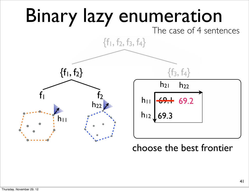
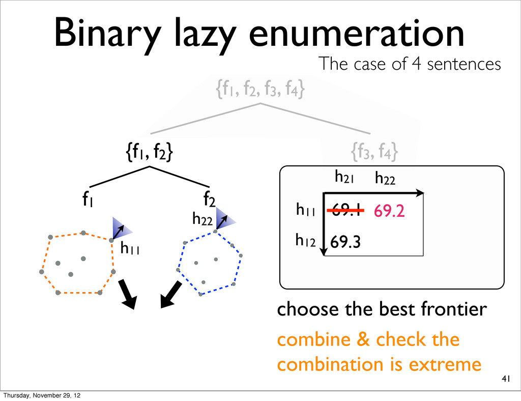
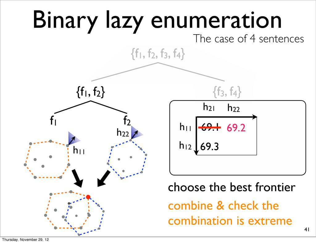
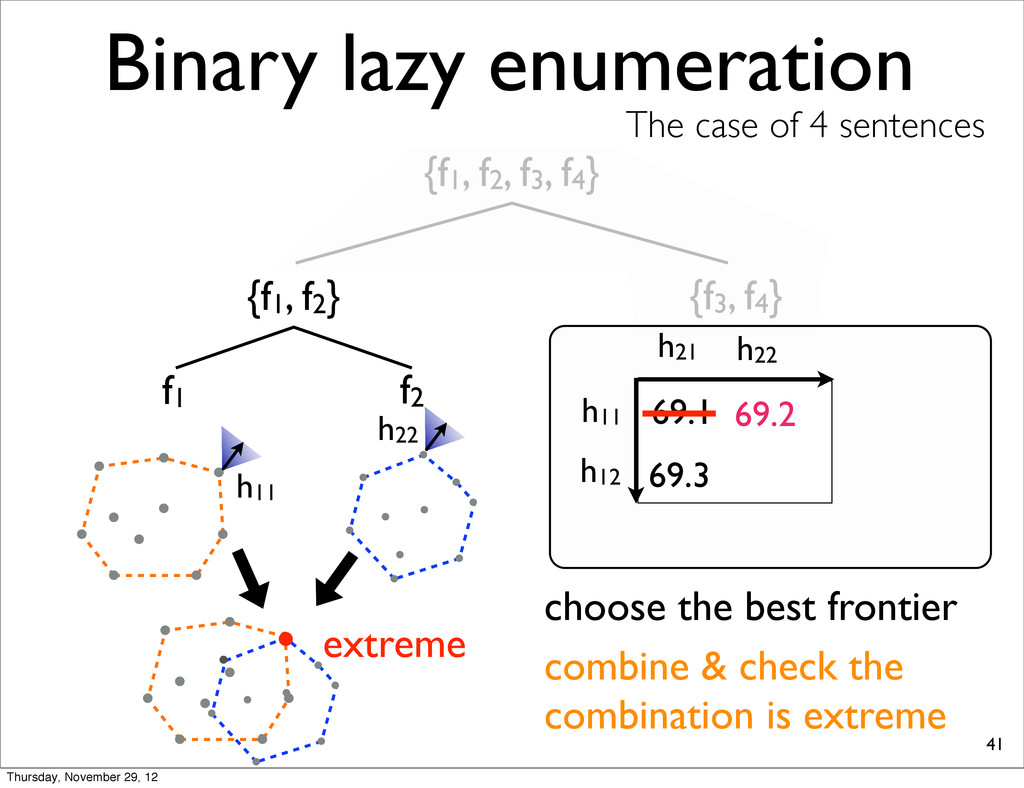
The case of 4 sentences {f1, f2} f1 f2 h11 h11 h21 69.1 choose the best frontier h22 69.2 h22 h12 69.3 combine & check the combination is extreme Thursday, November 29, 12
The case of 4 sentences {f1, f2} f1 f2 h11 h11 h21 69.1 choose the best frontier h22 69.2 h22 h12 69.3 combine & check the combination is extreme Thursday, November 29, 12
The case of 4 sentences {f1, f2} f1 f2 h11 h11 h21 69.1 choose the best frontier h22 69.2 h22 h12 69.3 combine & check the combination is extreme Thursday, November 29, 12
The case of 4 sentences {f1, f2} f1 f2 h11 h11 h21 69.1 choose the best frontier h22 69.2 h22 h12 69.3 combine & check the combination is extreme extreme Thursday, November 29, 12
The case of 4 sentences {f1, f2} f1 f2 h11 h11 h21 69.1 choose the best frontier h22 69.2 h22 h12 69.3 combine & check the combination is extreme extreme Thursday, November 29, 12
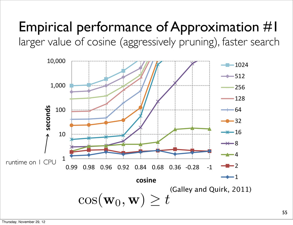
too many LPs to be solved. • Approximations #1: cos(w, w0) >= t - w0: reasonable approximation of ŵ by 1D-MERT • Approximations #2 - pruning the output of combined N-best lists by model score wrt wbest (best model on the entire tuning set) 46 Thursday, November 29, 12
exact LP-MERT - effect of number of features on runtime - scalability of the number of sentences. • evaluate LP-MERT w/ beam search - BLEU scores for dev set - end-to-end MERT comparison 48 Thursday, November 29, 12
cube pruning • task: WMT 2010 English-to-German - dev set: WMT 2009 test set - test set: WMT 2010 test set • features: 13 (use two language models) • N-best list size is 100 • evaluation: sentence BLEU (Lin & Och, 2004) 49 Thursday, November 29, 12
restarts and random walks (Moore & Quirk, 2008) - the values of the parameters they used in experiments are not clear from this paper. 50 Thursday, November 29, 12
1D-MERT are evaluated on the same combined N-best lists, even though running multiple iterations of MERT with either LP-MERT or 1D-MERT would normally produce different combined N-best lists.” -(Galley and Quirk, 2011) Thursday, November 29, 12
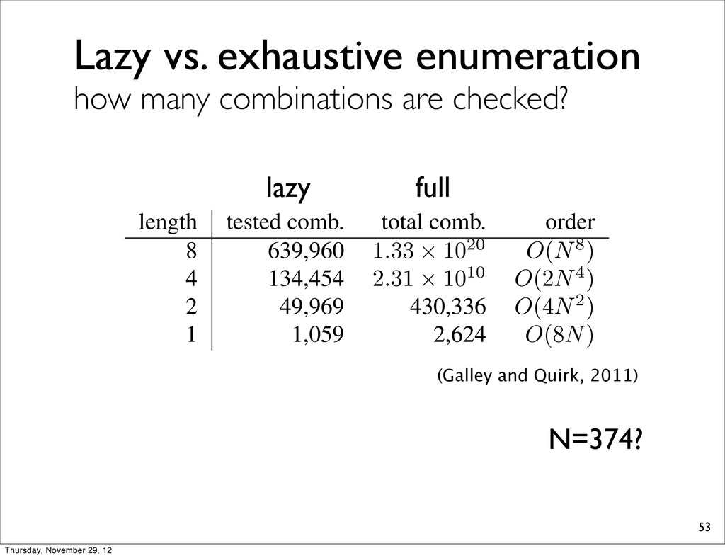
5 6 7 0 100 200 300 400 500 600 700 800 900 1000 S=8 S=4 S=2 BLEU[%] Figure 5: Line graph of sorted differences in BLEUn4r1 [%] scores between LP-MERT and 1D-MERT on 1000 tuning sets of size S = 2 , 4 , 8 . The highest differ- length 8 4 2 1 Table 1: N ments of F full comb number o (Galley and Quirk, 2011) 1000 overlapping subsets for S = 2, 4, and 8. experimented on 374-best lists after 5 iterations of MERT NOTE: x-coordinate is sorted by ΔBLEU LP-MERT is better 1D-MERT is better Thursday, November 29, 12
length tested comb. total comb. order 8 639,960 1 . 33 ⇥ 10 20 O ( N8 ) 4 134,454 2 . 31 ⇥ 10 10 O (2 N4 ) 2 49,969 430,336 O (4 N2 ) 1 1,059 2,624 O (8 N ) Table 1: Number of tested combinations for the experi- ments of Fig. 5. LP-MERT with S = 8 checks only 600K full combinations on average, much less than the total number of combinations (which is more than 10 20). (Galley and Quirk, 2011) N=374? full lazy Thursday, November 29, 12
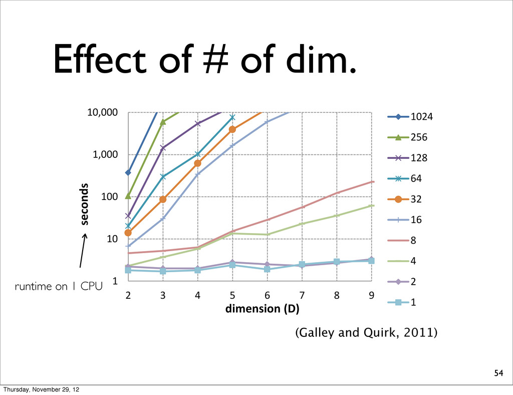
differ- 13.1. approx- g with a ual data. get side y data), ata (pri- develop- Table 1: Number of tested combinations for the experi- ments of Fig. 5. LP-MERT with S = 8 checks only 600K full combinations on average, much less than the total number of combinations (which is more than 10 20). 1 10 100 1,000 10,000 2 3 4 5 6 7 8 9 seconds 1024 256 128 64 32 16 8 4 2 1 dimension (D) Figure 6: Effect of the number of features (runtime on 1 CPU of a modern computer). Each curve represents a different number of tuning sentences. (Galley and Quirk, 2011) runtime on 1 CPU Thursday, November 29, 12
pruning), faster search 55 1 10 100 1,000 10,000 0.99 0.98 0.96 0.92 0.84 0.68 0.36 -0.28 -1 seconds 1024 512 256 128 64 32 16 8 4 2 1 cosine Figure 7: Effect of a constraint on w (runtime on 1 CPU). 32 64 128 256 512 1024 to hype challen the sea mate se Othe of grad simple et al., 2 search it still r flect, e suffers feature cos( w0, w ) t (Galley and Quirk, 2011) runtime on 1 CPU Thursday, November 29, 12
exact LP-MERT - effect of number of features on runtime - scalability of the number of sentences. • evaluate LP-MERT w/ beam search - BLEU scores for dev set - end-to-end MERT comparison 56 Thursday, November 29, 12
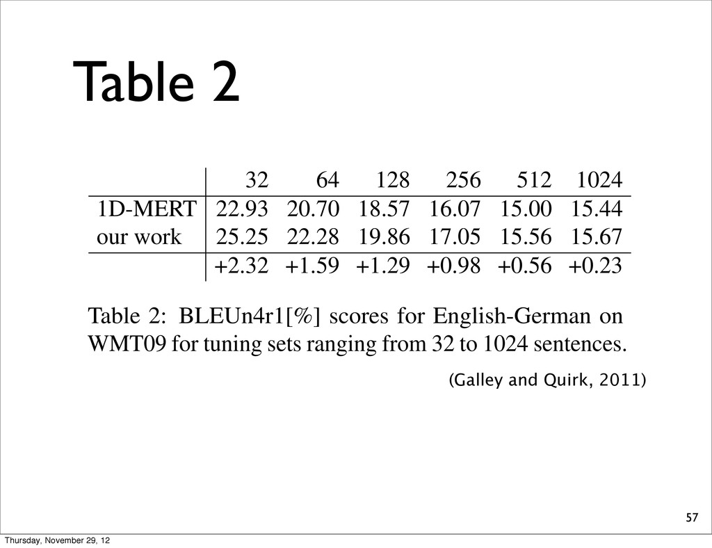
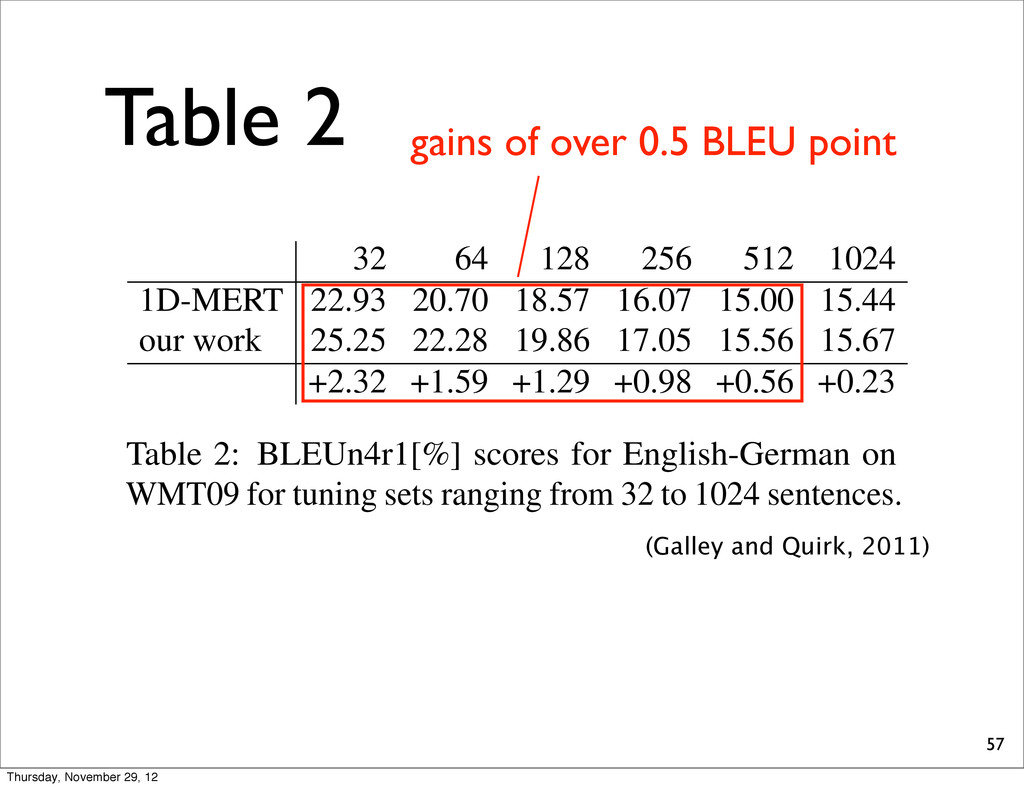
w (runtime on 1 CPU). 32 64 128 256 512 1024 1D-MERT 22.93 20.70 18.57 16.07 15.00 15.44 our work 25.25 22.28 19.86 17.05 15.56 15.67 +2.32 +1.59 +1.29 +0.98 +0.56 +0.23 Table 2: BLEUn4r1[%] scores for English-German on WMT09 for tuning sets ranging from 32 to 1024 sentences. size. Results are displayed in Table 2. The gains are fairly substantial, with gains of 0.5 BLEU point or more in all cases where S 512 .8 Finally, we perform an end-to-end MERT comparison, where et al., search it still flect, suffer featur diffic metho ramet We numb timiza in the weigh eter in ing th and st 2002) (Galley and Quirk, 2011) Thursday, November 29, 12
w (runtime on 1 CPU). 32 64 128 256 512 1024 1D-MERT 22.93 20.70 18.57 16.07 15.00 15.44 our work 25.25 22.28 19.86 17.05 15.56 15.67 +2.32 +1.59 +1.29 +0.98 +0.56 +0.23 Table 2: BLEUn4r1[%] scores for English-German on WMT09 for tuning sets ranging from 32 to 1024 sentences. size. Results are displayed in Table 2. The gains are fairly substantial, with gains of 0.5 BLEU point or more in all cases where S 512 .8 Finally, we perform an end-to-end MERT comparison, where et al., search it still flect, suffer featur diffic metho ramet We numb timiza in the weigh eter in ing th and st 2002) gains of over 0.5 BLEU point (Galley and Quirk, 2011) Thursday, November 29, 12
devset WMT 2010 test set 1D-MERT 9 15.97 16.91 LP-MERT 7 16.21 17.08 +0.24 +0.17 This table is created from the results of (Galley and Quirk, 2011) Thursday, November 29, 12
search • proposed LP-MERT, an exact search algorithm on N-best lists in the multi-dimensional case. - give us the optimal parameters as ground truth - In practice, two approximations are offered • Experimental results: slightly improves over Och’s MERT in terms of sentence BLEU. 59 Thursday, November 29, 12