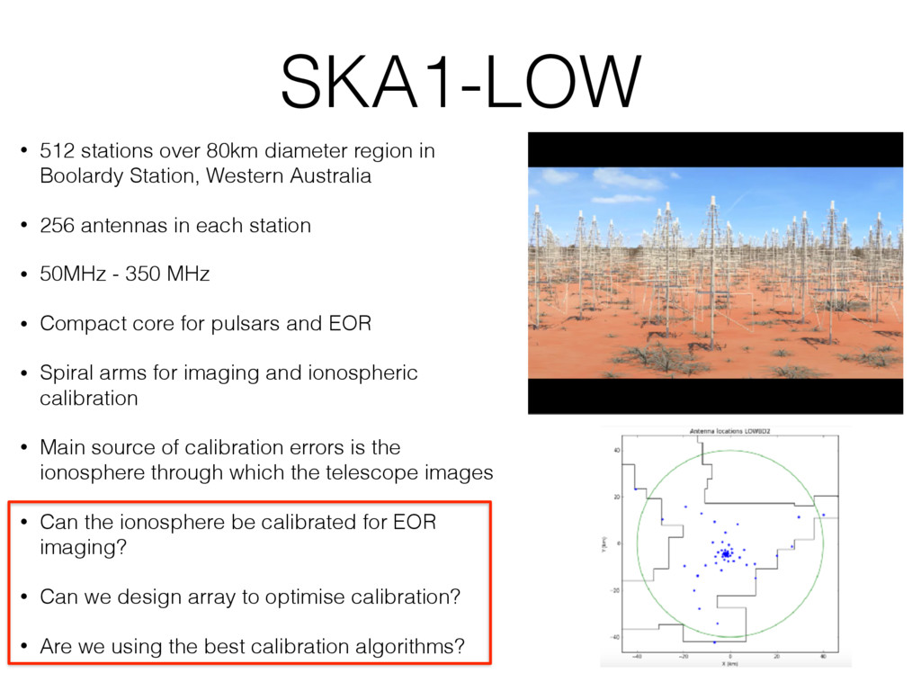
Station, Western Australia • 256 antennas in each station • 50MHz - 350 MHz • Compact core for pulsars and EOR • Spiral arms for imaging and ionospheric calibration • Main source of calibration errors is the ionosphere through which the telescope images • Can the ionosphere be calibrated for EOR imaging? • Can we design array to optimise calibration? • Are we using the best calibration algorithms?
Station, Western Australia • 256 antennas in each station • 50MHz - 350 MHz • Compact core for pulsars and EOR • Spiral arms for imaging and ionospheric calibration • Main source of calibration errors is the ionosphere through which the telescope images • Can the ionosphere be calibrated for EOR imaging? • Can we design array to optimise calibration? • Are we using the best calibration algorithms?
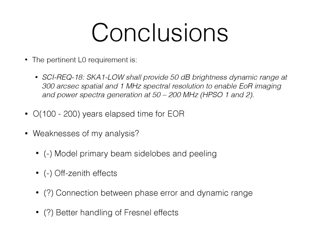
is: • SCI-REQ-18: SKA1-LOW shall provide 50 dB brightness dynamic range at 300 arcsec spatial and 1 MHz spectral resolution to enable EoR imaging and power spectra generation at 50 – 200 MHz (HPSO 1 and 2).
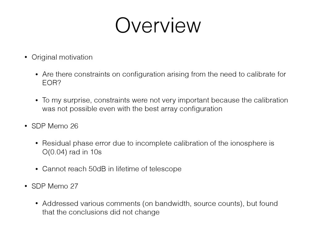
arising from the need to calibrate for EOR? • To my surprise, constraints were not very important because the calibration was not possible even with the best array configuration • SDP Memo 26 • Residual phase error due to incomplete calibration of the ionosphere is O(0.04) rad in 10s • Cannot reach 50dB in lifetime of telescope • SDP Memo 27 • Addressed various comments (on bandwidth, source counts), but found that the conclusions did not change
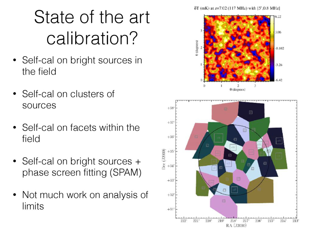
on clusters of sources • Self-cal on facets within the field • Self-cal on bright sources + phase screen fitting (SPAM) • Not much work on analysis of limits State of the art calibration?
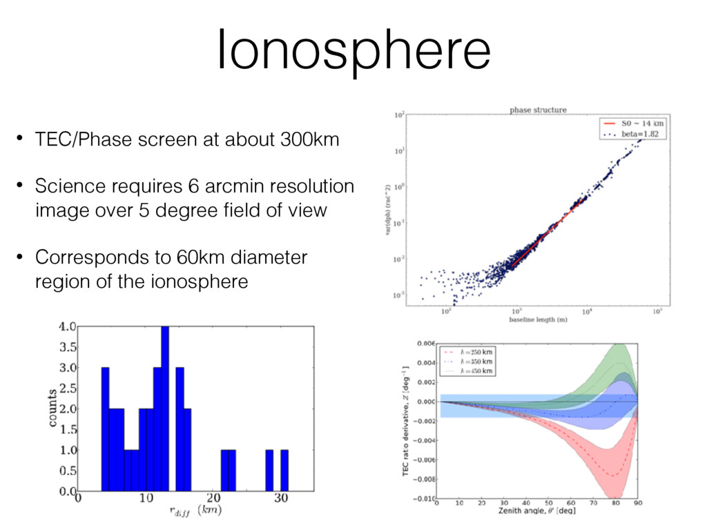
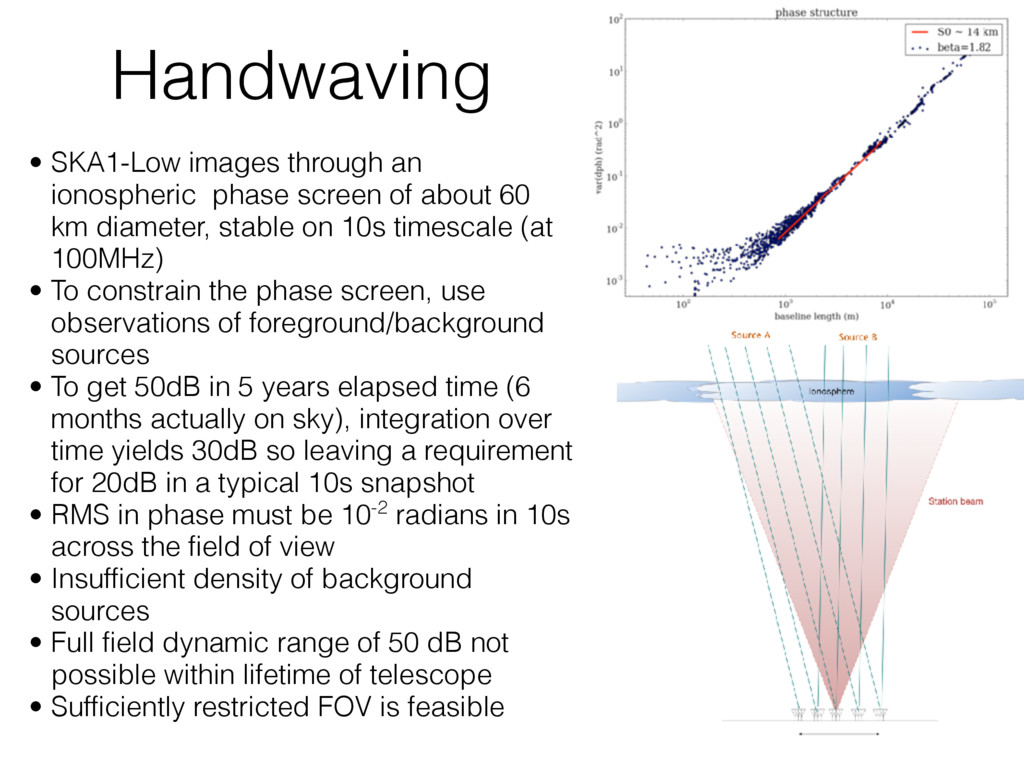
60 km diameter, stable on 10s timescale (at 100MHz) • To constrain the phase screen, use observations of foreground/background sources • To get 50dB in 5 years elapsed time (6 months actually on sky), integration over time yields 30dB so leaving a requirement for 20dB in a typical 10s snapshot • RMS in phase must be 10-2 radians in 10s across the field of view • Insufficient density of background sources • Full field dynamic range of 50 dB not possible within lifetime of telescope • Sufficiently restricted FOV is feasible Handwaving
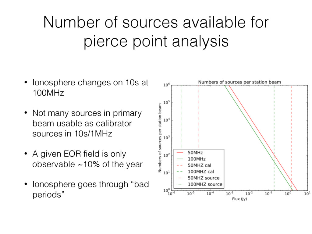
changes on 10s at 100MHz • Not many sources in primary beam usable as calibrator sources in 10s/1MHz • A given EOR field is only observable ~10% of the year • Ionosphere goes through “bad periods”
analysed the estimation of a single TID and found that to be well-conditioned • Not surprising: many, many fewer degrees of freedom in a sinusoid than the turbulent spectrum
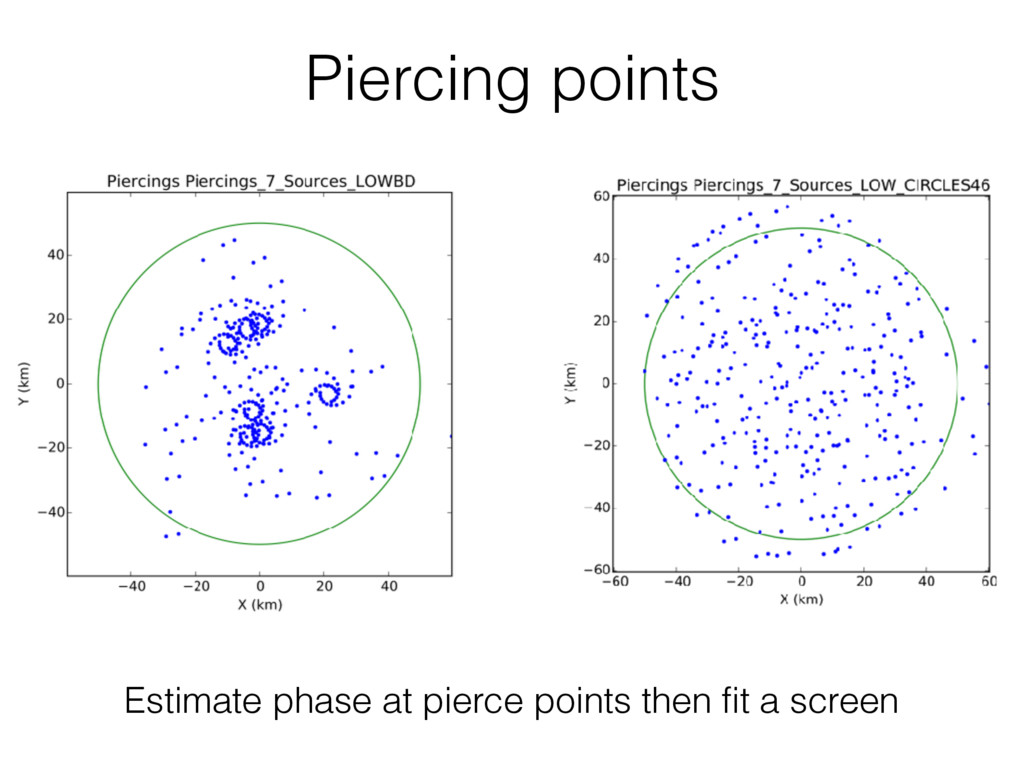
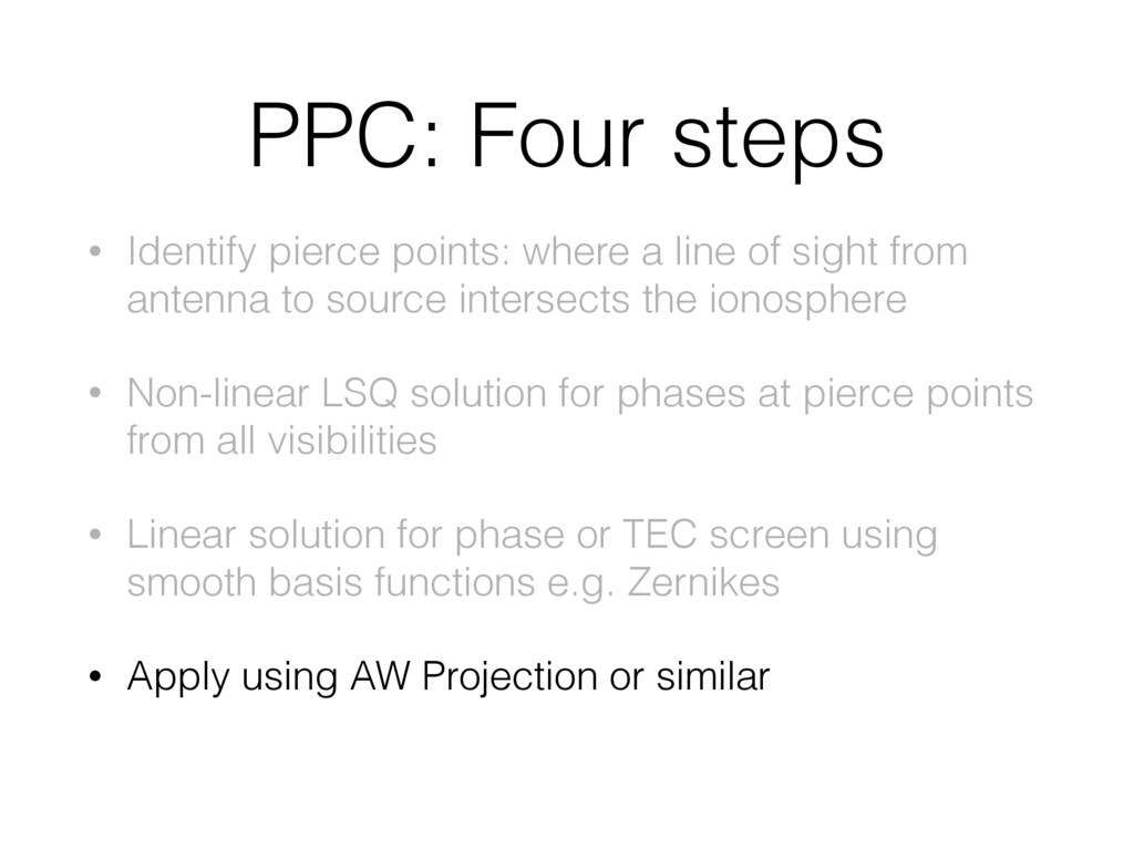
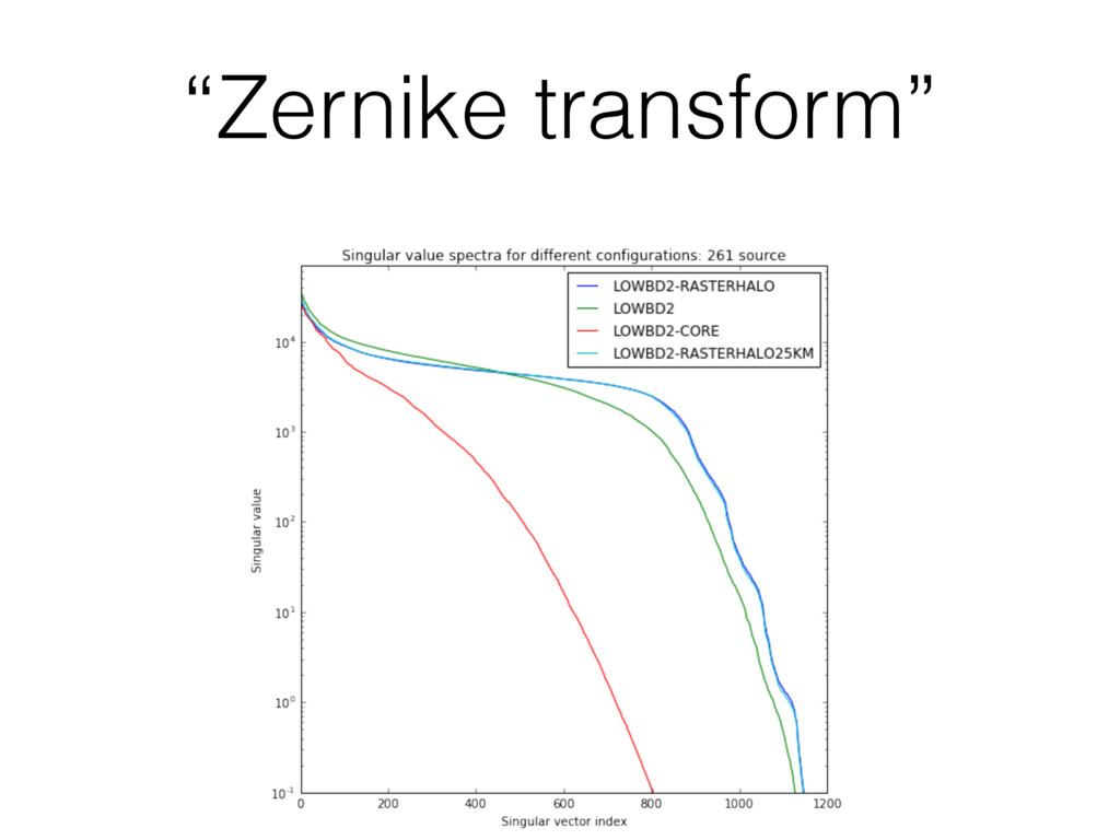
of sight from antenna to source intersects the ionosphere • Non-linear LSQ solution for phases at pierce points from all visibilities • Linear solution for phase or TEC screen using smooth basis functions e.g. Zernikes
of sight from antenna to source intersects the ionosphere • Non-linear LSQ solution for phases at pierce points from all visibilities • Linear solution for phase or TEC screen using smooth basis functions e.g. Zernikes • Apply using AW Projection or similar
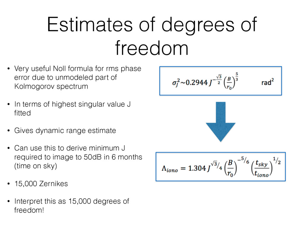
for rms phase error due to unmodeled part of Kolmogorov spectrum • In terms of highest singular value J fitted • Gives dynamic range estimate • Can use this to derive minimum J required to image to 50dB in 6 months (time on sky) • 15,000 Zernikes • Interpret this as 15,000 degrees of freedom!
• Use Bregman’s source counts in place of Condon’s. • Corrected errors in noise calculation using tabulations in BD V2 • Updated diffractive scale from 14km to 7km (per recently published LOFAR work) • Introduced superior ionosphere estimation approach
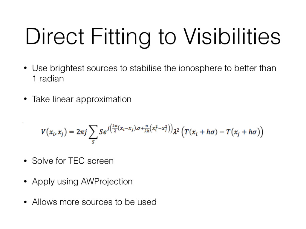
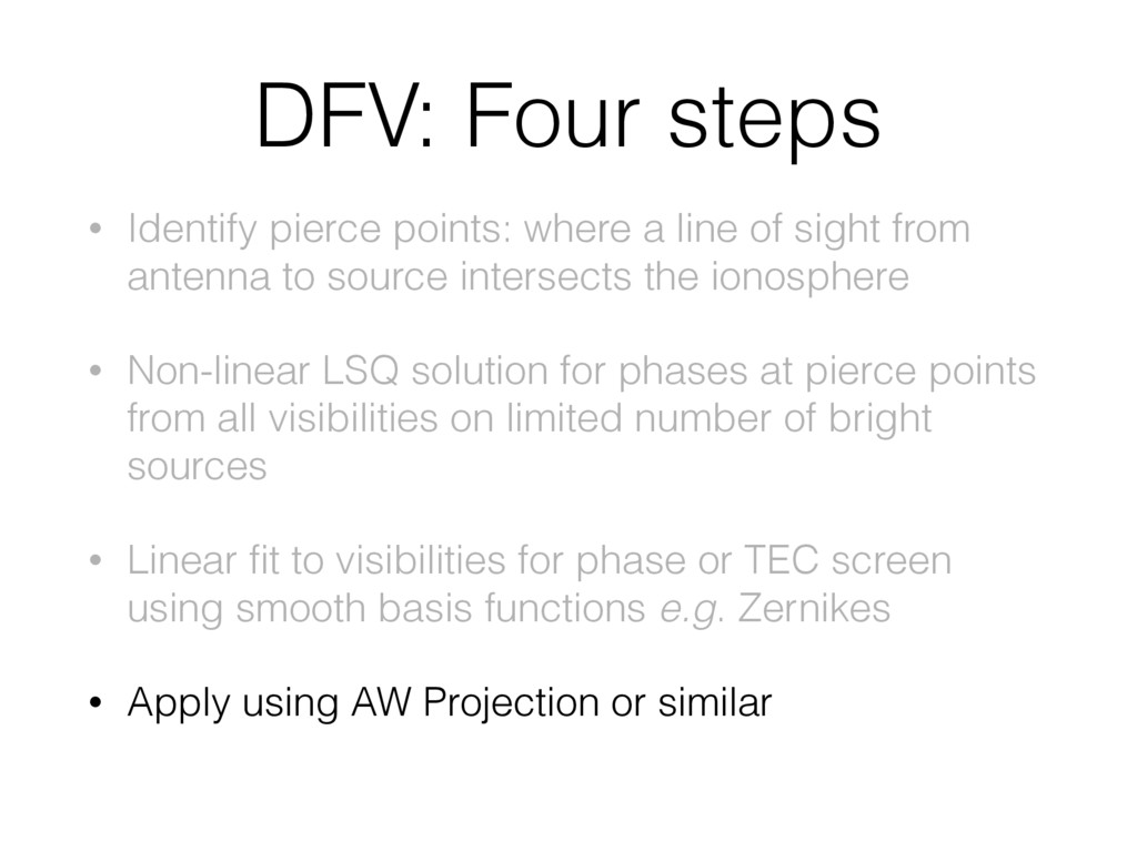
of sight from antenna to source intersects the ionosphere • Non-linear LSQ solution for phases at pierce points from all visibilities on limited number of bright sources
of sight from antenna to source intersects the ionosphere • Non-linear LSQ solution for phases at pierce points from all visibilities on limited number of bright sources • Linear fit to visibilities for phase or TEC screen using smooth basis functions e.g. Zernikes
of sight from antenna to source intersects the ionosphere • Non-linear LSQ solution for phases at pierce points from all visibilities on limited number of bright sources • Linear fit to visibilities for phase or TEC screen using smooth basis functions e.g. Zernikes • Apply using AW Projection or similar
shall provide 50 dB brightness dynamic range at 300 arcsec spatial and 1 MHz spectral resolution to enable EoR imaging and power spectra generation at 50 – 200 MHz (HPSO 1 and 2). • O(100 - 200) years elapsed time for EOR • Weaknesses of my analysis? • (-) Model primary beam sidelobes and peeling • (-) Off-zenith effects • (?) Connection between phase error and dynamic range • (?) Better handling of Fresnel effects
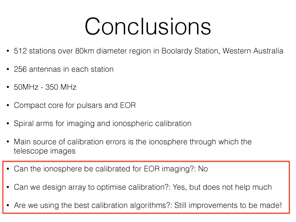
Station, Western Australia • 256 antennas in each station • 50MHz - 350 MHz • Compact core for pulsars and EOR • Spiral arms for imaging and ionospheric calibration • Main source of calibration errors is the ionosphere through which the telescope images • Can the ionosphere be calibrated for EOR imaging?: No • Can we design array to optimise calibration?: Yes, but does not help much • Are we using the best calibration algorithms?: Still improvements to be made!
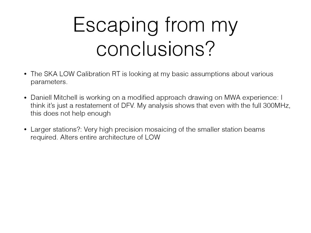
is looking at my basic assumptions about various parameters. • Daniell Mitchell is working on a modified approach drawing on MWA experience: I think it’s just a restatement of DFV. My analysis shows that even with the full 300MHz, this does not help enough
is looking at my basic assumptions about various parameters. • Daniell Mitchell is working on a modified approach drawing on MWA experience: I think it’s just a restatement of DFV. My analysis shows that even with the full 300MHz, this does not help enough • Larger stations?: Very high precision mosaicing of the smaller station beams required. Alters entire architecture of LOW
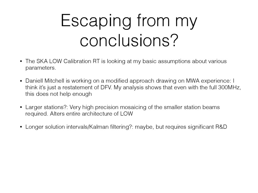
is looking at my basic assumptions about various parameters. • Daniell Mitchell is working on a modified approach drawing on MWA experience: I think it’s just a restatement of DFV. My analysis shows that even with the full 300MHz, this does not help enough • Larger stations?: Very high precision mosaicing of the smaller station beams required. Alters entire architecture of LOW • Longer solution intervals/Kalman filtering?: maybe, but requires significant R&D
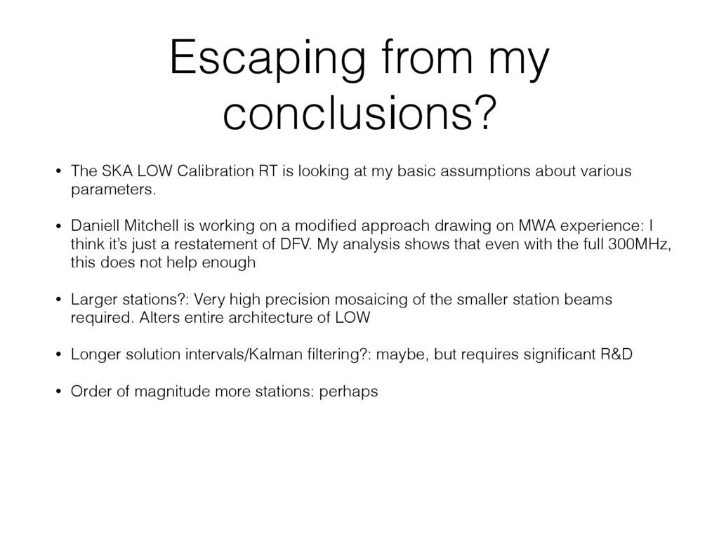
is looking at my basic assumptions about various parameters. • Daniell Mitchell is working on a modified approach drawing on MWA experience: I think it’s just a restatement of DFV. My analysis shows that even with the full 300MHz, this does not help enough • Larger stations?: Very high precision mosaicing of the smaller station beams required. Alters entire architecture of LOW • Longer solution intervals/Kalman filtering?: maybe, but requires significant R&D • Order of magnitude more stations: perhaps
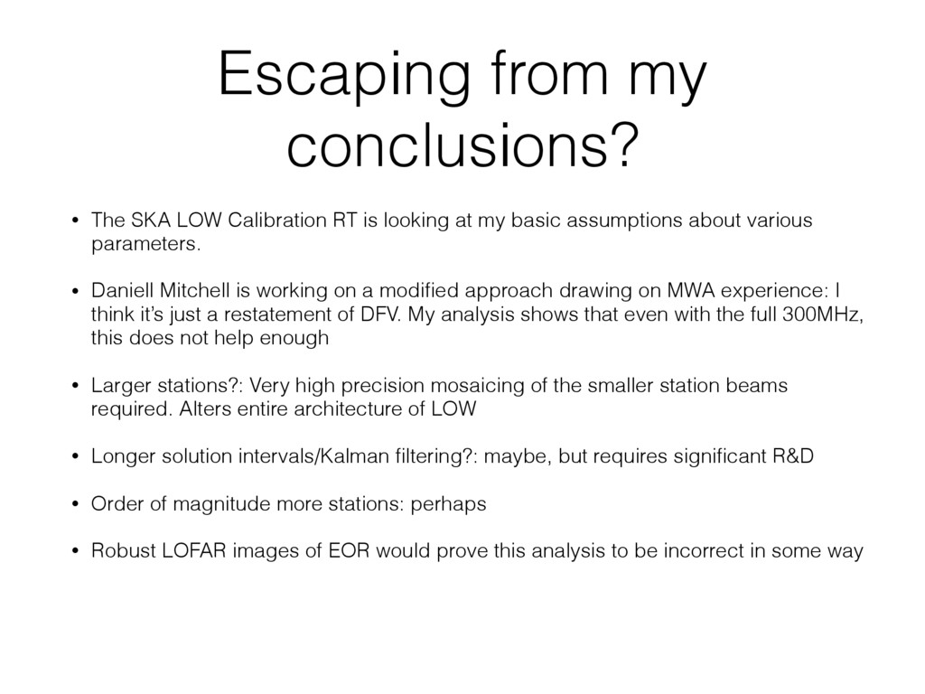
is looking at my basic assumptions about various parameters. • Daniell Mitchell is working on a modified approach drawing on MWA experience: I think it’s just a restatement of DFV. My analysis shows that even with the full 300MHz, this does not help enough • Larger stations?: Very high precision mosaicing of the smaller station beams required. Alters entire architecture of LOW • Longer solution intervals/Kalman filtering?: maybe, but requires significant R&D • Order of magnitude more stations: perhaps • Robust LOFAR images of EOR would prove this analysis to be incorrect in some way
is looking at my basic assumptions about various parameters. • Daniell Mitchell is working on a modified approach drawing on MWA experience: I think it’s just a restatement of DFV. My analysis shows that even with the full 300MHz, this does not help enough • Larger stations?: Very high precision mosaicing of the smaller station beams required. Alters entire architecture of LOW • Longer solution intervals/Kalman filtering?: maybe, but requires significant R&D • Order of magnitude more stations: perhaps • Robust LOFAR images of EOR would prove this analysis to be incorrect in some way • I would like to encourage more work in this analytical vein.
of data processing rather than just work on algorithms themselves • The calibration of LOW is intrinically difficult to understand and analyse • My work is on the right track but requires further extension either in the current framework or in somethin more sophisticated • Lots of opportunities for this audience!