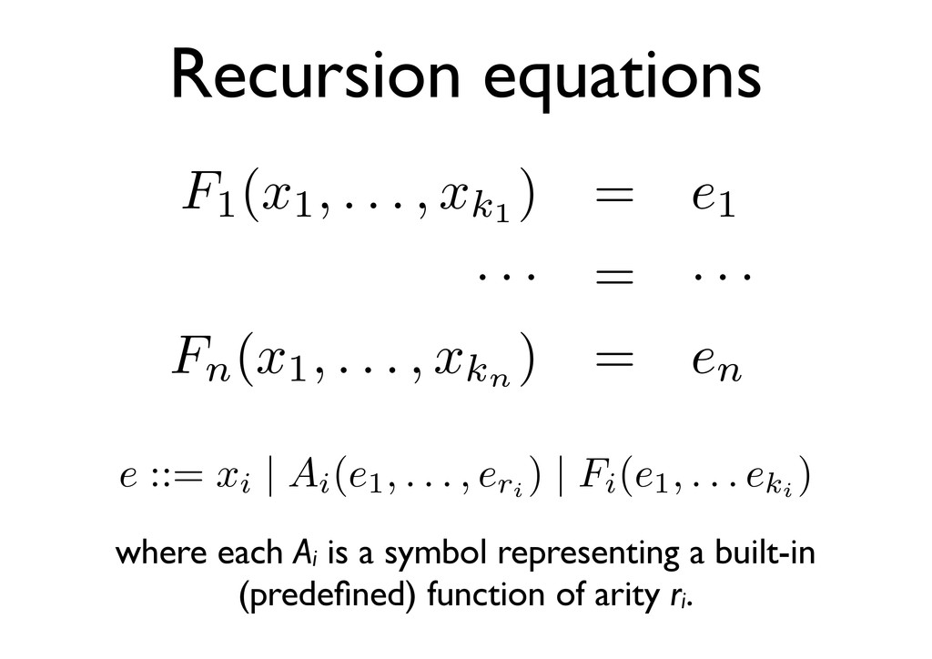
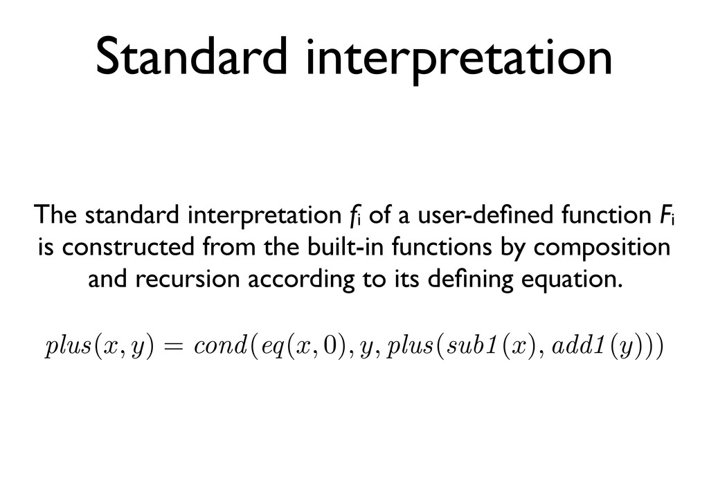
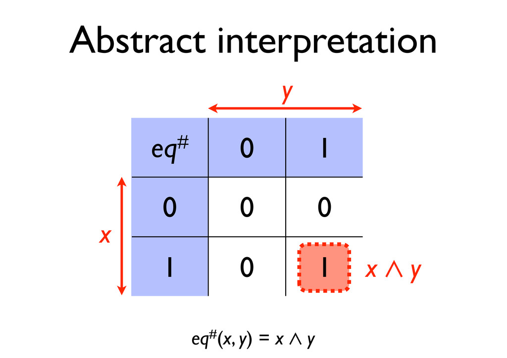
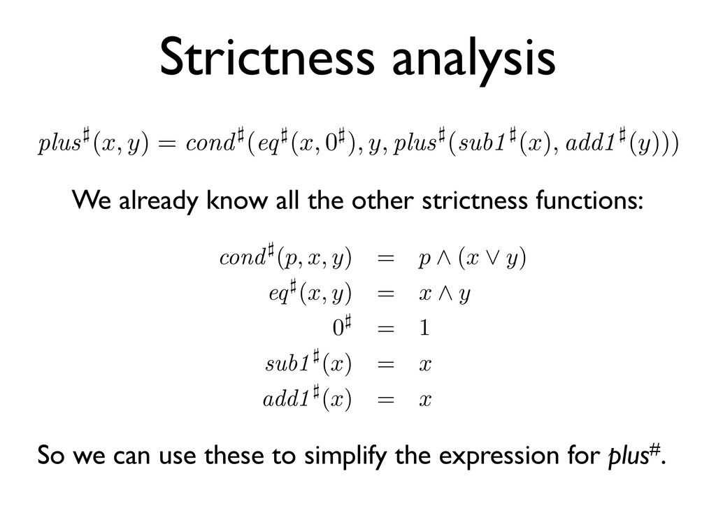
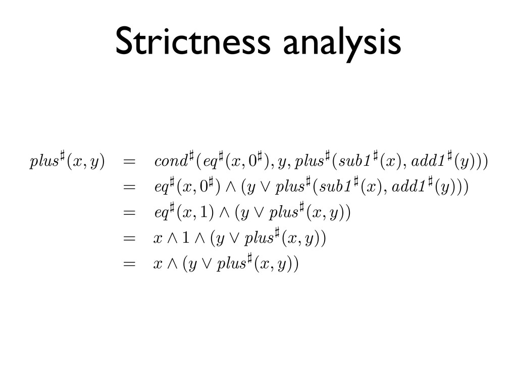
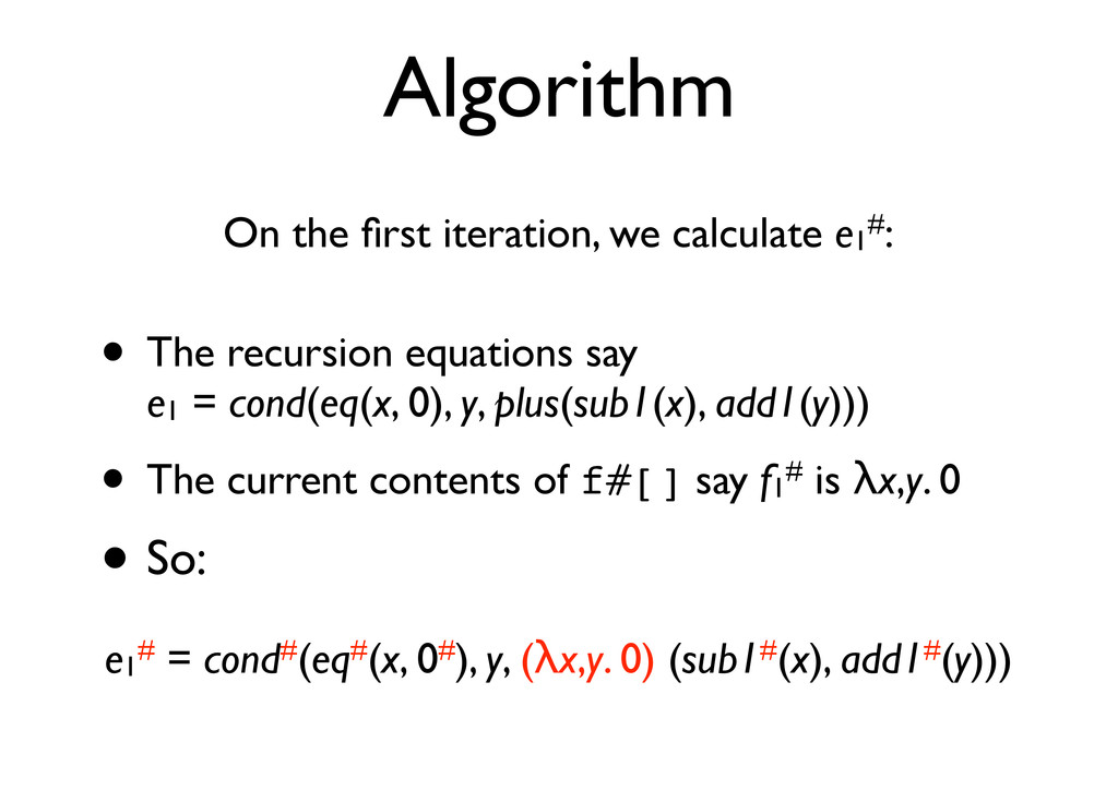
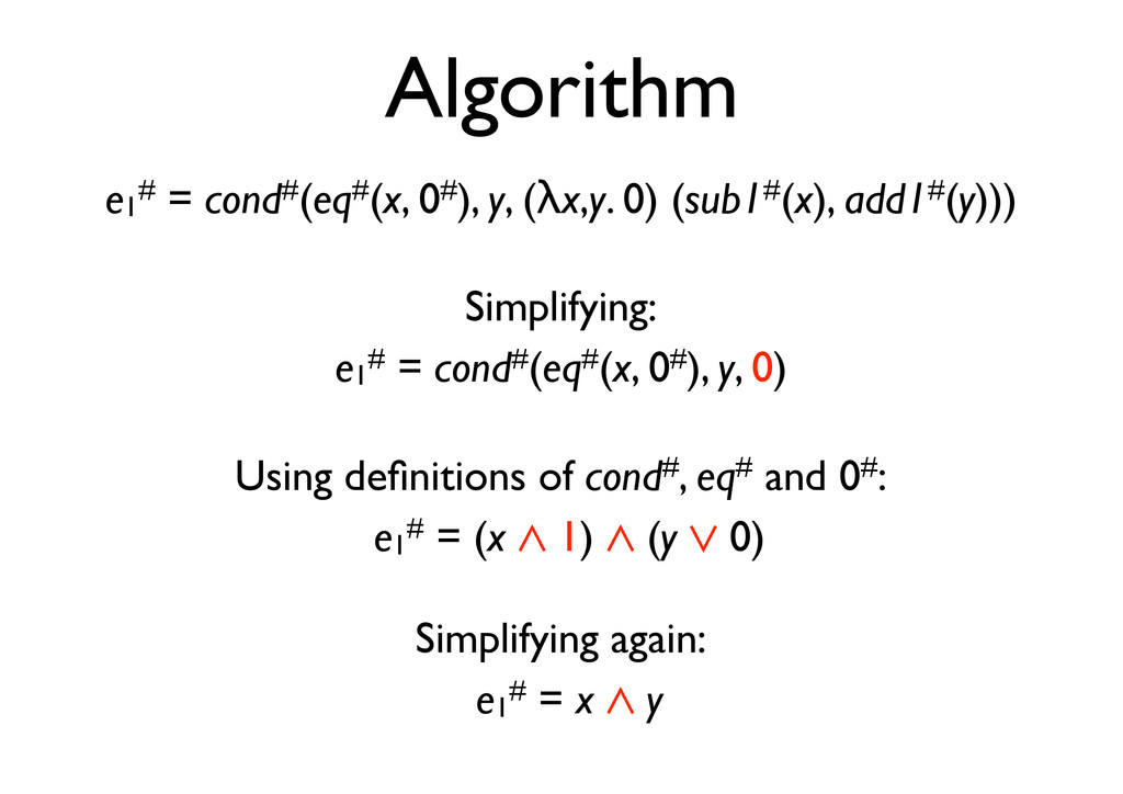
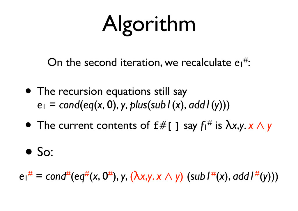
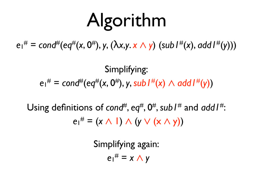
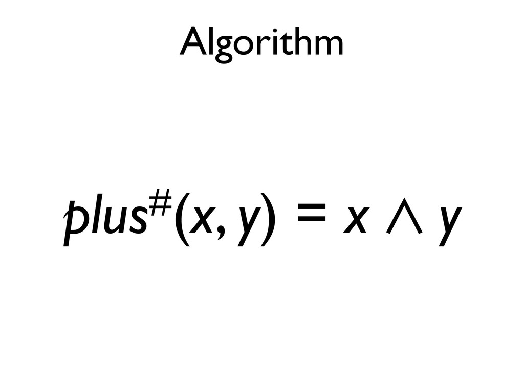
), y, plus (sub1 (x), add1 (y))) = eq (x, 0 ) ∧ (y ∨ plus (sub1 (x), add1 (y))) = eq (x, 1) ∧ (y ∨ plus (x, y)) = x ∧ 1 ∧ (y ∨ plus (x, y)) = x ∧ (y ∨ plus (x, y)) plus (x, y) = cond (eq (x, 0 ), y, plus (sub1 (x), add1 (y))) = eq (x, 0 ) ∧ (y ∨ plus (sub1 (x), add1 (y))) = eq (x, 1) ∧ (y ∨ plus (x, y)) = x ∧ 1 ∧ (y ∨ plus (x, y)) = x ∧ (y ∨ plus (x, y)) plus (x, y) = cond (eq (x, 0 ), y, plus (sub1 (x), add1 (y))) = eq (x, 0 ) ∧ (y ∨ plus (sub1 (x), add1 (y))) = eq (x, 1) ∧ (y ∨ plus (x, y)) = x ∧ 1 ∧ (y ∨ plus (x, y)) = x ∧ (y ∨ plus (x, y)) plus (x, y) = cond (eq (x, 0 ), y, plus (sub1 (x), add1 (y))) = eq (x, 0 ) ∧ (y ∨ plus (sub1 (x), add1 (y))) = eq (x, 1) ∧ (y ∨ plus (x, y)) = x ∧ 1 ∧ (y ∨ plus (x, y)) = x ∧ (y ∨ plus (x, y)) plus (x, y) = cond (eq (x, 0 ), y, plus (sub1 (x), add1 (y))) = eq (x, 0 ) ∧ (y ∨ plus (sub1 (x), add1 (y))) = eq (x, 1) ∧ (y ∨ plus (x, y)) = x ∧ 1 ∧ (y ∨ plus (x, y)) = x ∧ (y ∨ plus (x, y))
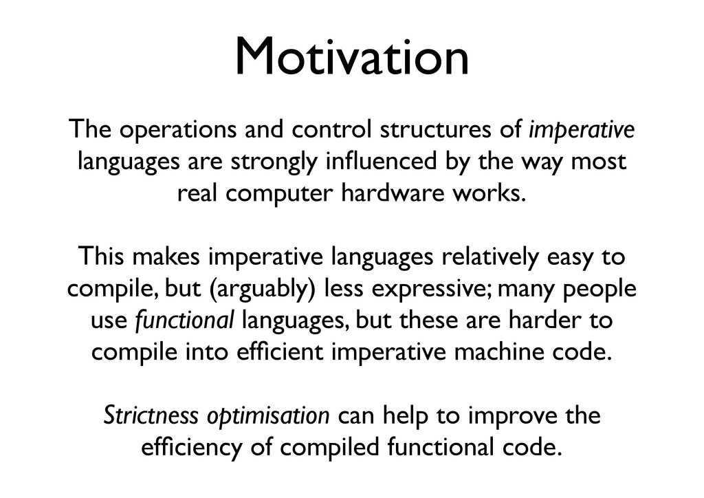
![Call-by-value evaluation e2 ⇓ v2 e1 [v2 /x] ⇓ v1](https://files.speakerdeck.com/presentations/4ea521c615006a005100a8e9/slide_1.jpg)
![Call-by-name evaluation e1 [e2 /x] ⇓ v (λx.e1 ) e2](https://files.speakerdeck.com/presentations/4ea521c615006a005100a8e9/slide_2.jpg)
![Algorithm for i = 1 to n do f#[i] :=](https://files.speakerdeck.com/presentations/4ea521c615006a005100a8e9/slide_33.jpg)
![Algorithm So, at the end of the first iteration, f#[1]](https://files.speakerdeck.com/presentations/4ea521c615006a005100a8e9/slide_37.jpg)
![Algorithm So, at the end of the second iteration, f#[1]](https://files.speakerdeck.com/presentations/4ea521c615006a005100a8e9/slide_40.jpg)