Interpreting Multiple Regression via an Ellipse Inscribed in a Square Extensible to Any Finite Dimensionality

Transcript

1. Interpreting Multiple Regression via an Ellipse Inscribed in a Square Extensible to any Finite Dimensionality 2019-08-14 Toshiyuki Shimono DSSV 2019 @ Kyoto , Japan 1
2. The main content 1. The multiple regression can be interpreted using an ellipse or (hyper) ellipsoid in a Euclid space. Ø Multiple corr. coeff. : Lengths ratio of line segments. Ø Regression coeff. : Read by a linear scholar field. Ø Partial corr. coeff : Read by a measure inside ellips-e/oid. 2. The above results makes : Ø Easy to understand/interpret the multiple regression both in (1) numerical results and (2) how to calculate. Ø may help in solving many paradoxical phenomena in multiple regression such as : multicollinearity, instability, etc. 2
3. I. Background 3 slides About Multiple Regressions 3
4. Linear Combination Modeling is Widely Used. Y = a1 X1 + … + ad Xd + b + error. Ø Many statistical models. Ø Multiple Regression. Ø Components of Deep Learning. Ø .. etc. 4
5. The Multiple Regression : → Regression coeff. ai → Multiple corr. coeff. ∈ [0,1] → Partial corr. coeff. ∈ [-1,1] ˆ Y = a 1 X 1 + a 2 X 2 +..+ a d X d + b 5
6. 6 The formulas above are obtained from [Kei Takeuchi, Haruo Yanai Tahenryou Kaiseki No Kiso. Tokyo Keizai Inc. (1972) ].
7. Results by Multiple Regression is, However, Difficult to Interpret : 1. Multiple correlation coefficient : Ø Difficult to know when/how it has unexpectedly large value. 2. Regression coefficients for Xi often can have : Ø different in ʶ signs from intuition. Ø very larger values from intuition. 3. Partial correlation coefficient for Xi : Ø can differ in ʶ signs from the corr. coeff. btw. Xi and Y. n Other issues: Ø Multicollinearity, especially for time series analysis. Ø Instability occurs w.r.t. sample from same population. Ø Incomputability by negative definite correlation matrix during handling missing values. 7 L
8. II. New 3 Theorems 7 slides How to Interpret the Results of Multiple Regression Geometrically. 8
9. Draw S, E and P (square, ellipse, point) When d = 2 : O P E(ellipse) S (square) When d = 3 : R X ×X for E ∩ S R X ×Y for P (1,1) (1,−1) (−1,−1) (−1,1) 9 S(cube) E(ellipsoid)
10. [Prep] Square S, Ellipse E, Point P 1. Define d (the number of explanatory variables) and set up an d-dim Euclid space (axes by: x1,.., xd). 2. Draw S : surrounded by x1 =±1, x2 =±1 .. xd =±1. 3. Ellipse E inscribing S centering the origin O=(0,..,0) : inscribed with the points C1, C2,..,Cd obtained from the d x d correlation matrix over X1,.., Xd as split into (C1|C2|..|Cd). 4. Point P inside E : whose i-th coordinate is specified by the correlation coefficient between Xi and Y. 10
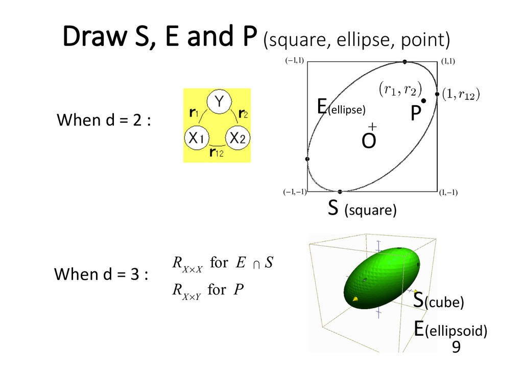
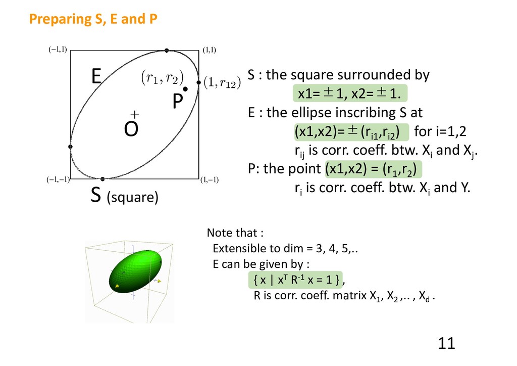
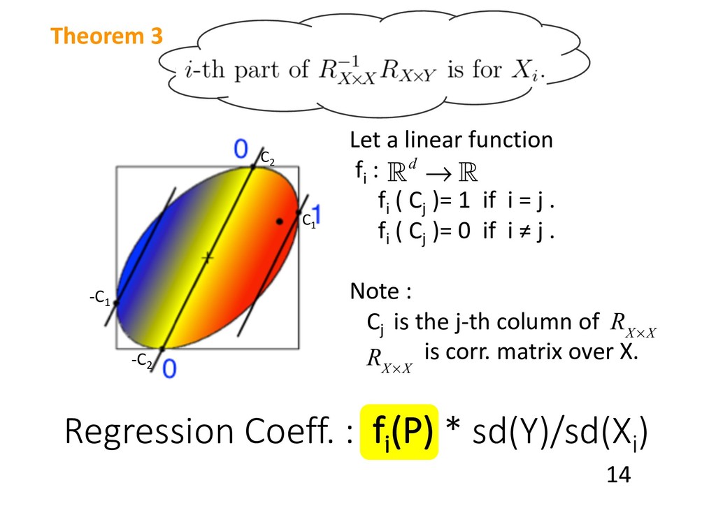
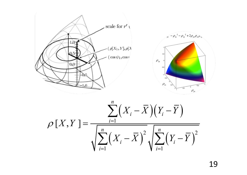
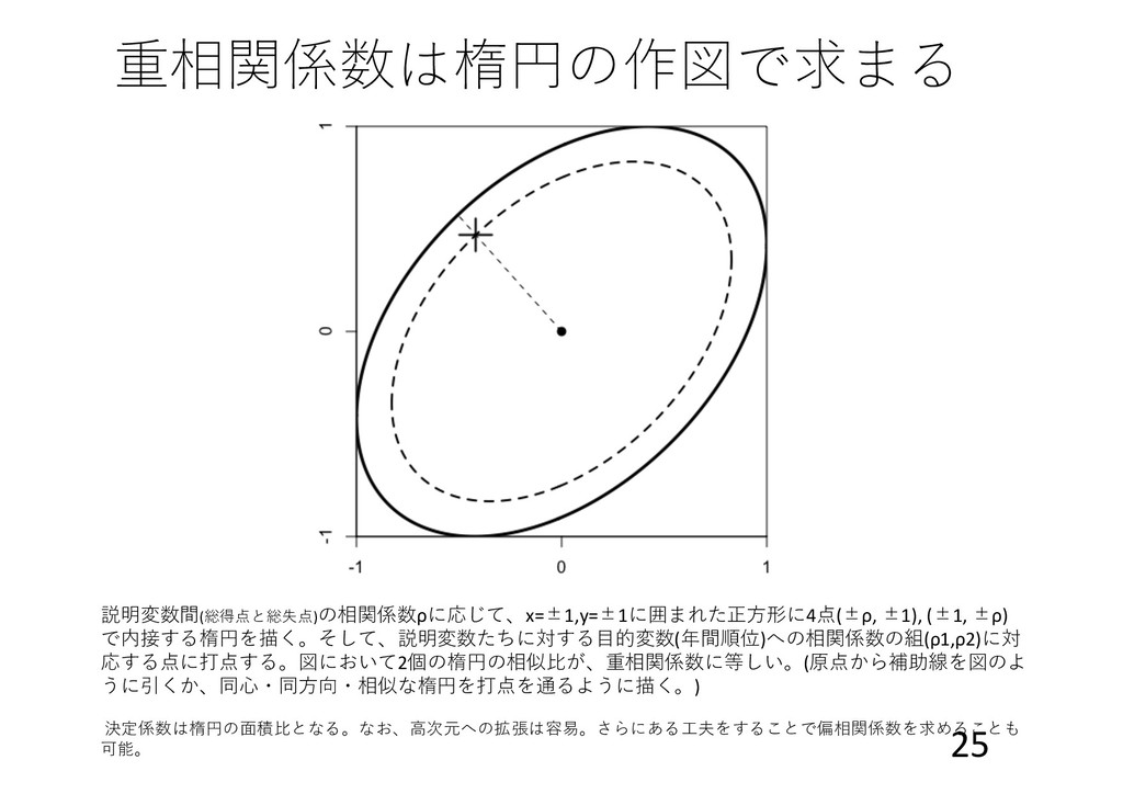
11. O P E S (square) (1,1) (1,−1) (−1,−1) (−1,1) S : the square surrounded by x1=±1, x2=±1. E : the ellipse inscribing S at (x1,x2)=±(ri1 ,ri2 ) for i=1,2 rij is corr. coeff. btw. Xi and Xj . P: the point (x1,x2) = (r1 ,r2 ) ri is corr. coeff. btw. Xi and Y. Note that : Extensible to dim = 3, 4, 5,.. E can be given by : { x | xT R-1 x = 1 } , R is corr. coeff. matrix X1 , X2 ,.. , Xd . 11 Preparing S, E and P
12. Multiple Corr. Coeff. = |OP|/|OP’| P P’ O P P’ O P P’ O P P’ O 12 Theorem 1
13. zz Partial Correlation : gi -1(P) Let a rod Pi- Pi+ be the longest one inside the ellipse E, passing through P, parallel to xi -axis with the same direction. Let an affine func. gi :R→Rd satisfy gi (Pi ±)=±1. Pi - Pi + P 13 Theorem 2 ! → !d
14. Regression Coeff. : fi (P) * sd(Y)/sd(Xi ) Let a linear function fi : Rd→R fi ( Cj )= 1 if i = j . fi ( Cj )= 0 if i ≠ j . Note : Cj is the j-th column of is corr. matrix over X. C1 C2 -C2 -C1 R X ×X R X ×X 14 Theorem 3 !d → !
15. Geometric 3 Theorems (novel): 1. Multiple corr. coeff. : It is |OP|/|OP’| by letting OP and E cross at P’. 2. [ Regression coeff. :] ai is fi (P) * sd(Y)/sd(Xi ) ← sd: standard deviation by letting linear functions fi : Rd→R as fi ( Cj )=δij (δij : Kronecker delta) for i, j∈{1,2,..,d}. 3. Partial corr. coeff. : Let a line segment Pi- Pi+ be the longest one inside E and parallel to xi -axis with the same direction. Fixing variables X1 , .., Xd except Xi , the partial corr. coeff. btw. Xi and Y is gi -1(P) by letting affine func. gi :R→Rd satisfy gi (Pi ±)=±1. 15
16. Usefulness of Theorems: ü The results of the multiple regression can be visualized in an easily understandable way when d = 2 or 3. ü The theorems may exploit new theories about linear combination modeling, which solve: Ø the interpretation of numerical computation results, Ø unstableness, Ø multicollinearity, Ø etc. 16 J
17. III. Proof Outlines 1. For d=2 2. Matrix Representation 3. Ellipsoid Expansion. 17
18. 予備スライド 18
19. ( )( ) ( ) ( ) 1 2 2 1 1 [ , ] n i i i n n i i i i X X Y Y X Y X X Y Y r = = = - - = - - å å å 19
20. 年間総得点と年間順位の関係 相関係数は -0.419.. 年間の得点が多いほど 順位は上がり優勝に近づく 20
21. 年間総失点と年間順位の関係 相関係数は +0.471.. 年間の失点が少ないほど 順位は上がり優勝に近づく 21
22. 総得点(x)と総失点(y)の関係 相関係数は +0.423.. (得点と失点は正に相関す る) 22
23. 順位を総得点と総失点で重回 帰 重相関係数は 0.828.. ◎⽬的変数(順位)は2個の説明変数を⽤いることで 予測精度が上がった。 ˕ ͜ΕΒͷ਺ྔͷؔ܎ΛͲ͏ཧղͨ͠Βྑ͍ͩΖ͏͔?? 23
24. ਺ྔͷؔ܎ΛͲ͏ཧղͨ͠Β ྑ͍ͩΖ͏͔?? • 実は、難しい数式を経由しなくても、重相関係数などは 作図で求めることができる。 • 重回帰の幾何的な表現により、把握が容易になる。 (この後で述べる⽅法を広く普及させたい!) • 重回帰に関係するいろいろな現象の理解を俯瞰的に与え ることが出来る。 • 既にある多変量に関係する理論を分かりやすく再構築す る可能性がある。 • 新たな理論を導く可能性もある。 24
25. 重相関係数は楕円の作図で求まる 説明変数間(総得点と総失点)の相関係数ρに応じて、x=±1,y=±1に囲まれた正⽅形に4点(±ρ, ±1), (±1, ±ρ) で内接する楕円を描く。そして、説明変数たちに対する⽬的変数(年間順位)への相関係数の組(ρ1,ρ2)に対 応する点に打点する。図において2個の楕円の相似⽐が、重相関係数に等しい。(原点から補助線を図のよ うに引くか、同⼼・同⽅向・相似な楕円を打点を通るように描く。) 決定係数は楕円の⾯積⽐となる。なお、⾼次元への拡張は容易。さらにある⼯夫をすることで偏相関係数を求めることも 可能。 25
26. 今後のスライドの構築案 • これまでのスライドの途中に絵を載せる • 証明のパートを後ろに続ける。 26