Semi-supervised Learning Approaches For Microstructure Classification Courtney Kunselman1, Vahid Attari1, Levi McClenny2, Ulisses Braga-Neto2, Raymundo Arroyavea1,3 1Department of Materials Science and Engineering, Texas A&M University 2Department of Electrical Engineering, Texas A&M University 3Department of Mechanical Engineering, Texas A&M University CHiMaD Workshop April 21, 2020
2 It is all about exploration! Mars 2020 is a Mars rover mission by NASA's Mars Exploration Program that includes the Perseverance rover with a planned launch on 17 July 2020, and touch down in Jezero crater on Mars on 18 February 2021.
3 Why? • 1st element: Acceleration of materials development and deployment • 2nd element: The creation and curation of large scale materials databases has been widely cited as a critical required component for the acceleration of materials development and deployment. – [Niezgoda et al. 2013] • This has been a recognized need by the materials community since the 1970’s . – [Materials Science and Engineering -- Volume II, The Needs, Priorities, and Opportunities for Materials Research] • 3rd element: Forging these links requires quantitative analysis, and while processing parameters and property observations are generally easily quantifiable—they tend to be represented as objects that exist in a relatively low dimensional space – [Kunselman et al. 2019] The need Solution Develop Improve
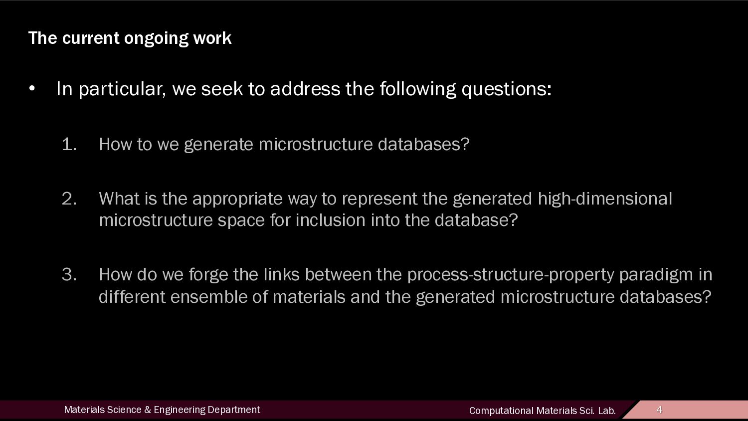
4 The current ongoing work • In particular, we seek to address the following questions: 1. How to we generate microstructure databases? 2. What is the appropriate way to represent the generated high-dimensional microstructure space for inclusion into the database? 3. How do we forge the links between the process-structure-property paradigm in different ensemble of materials and the generated microstructure databases?
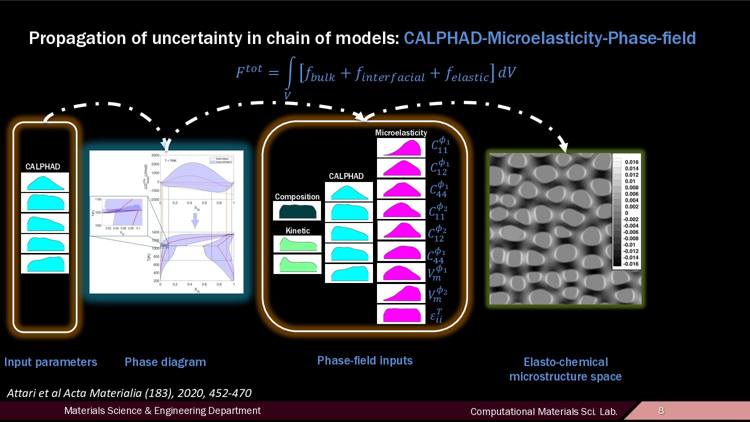
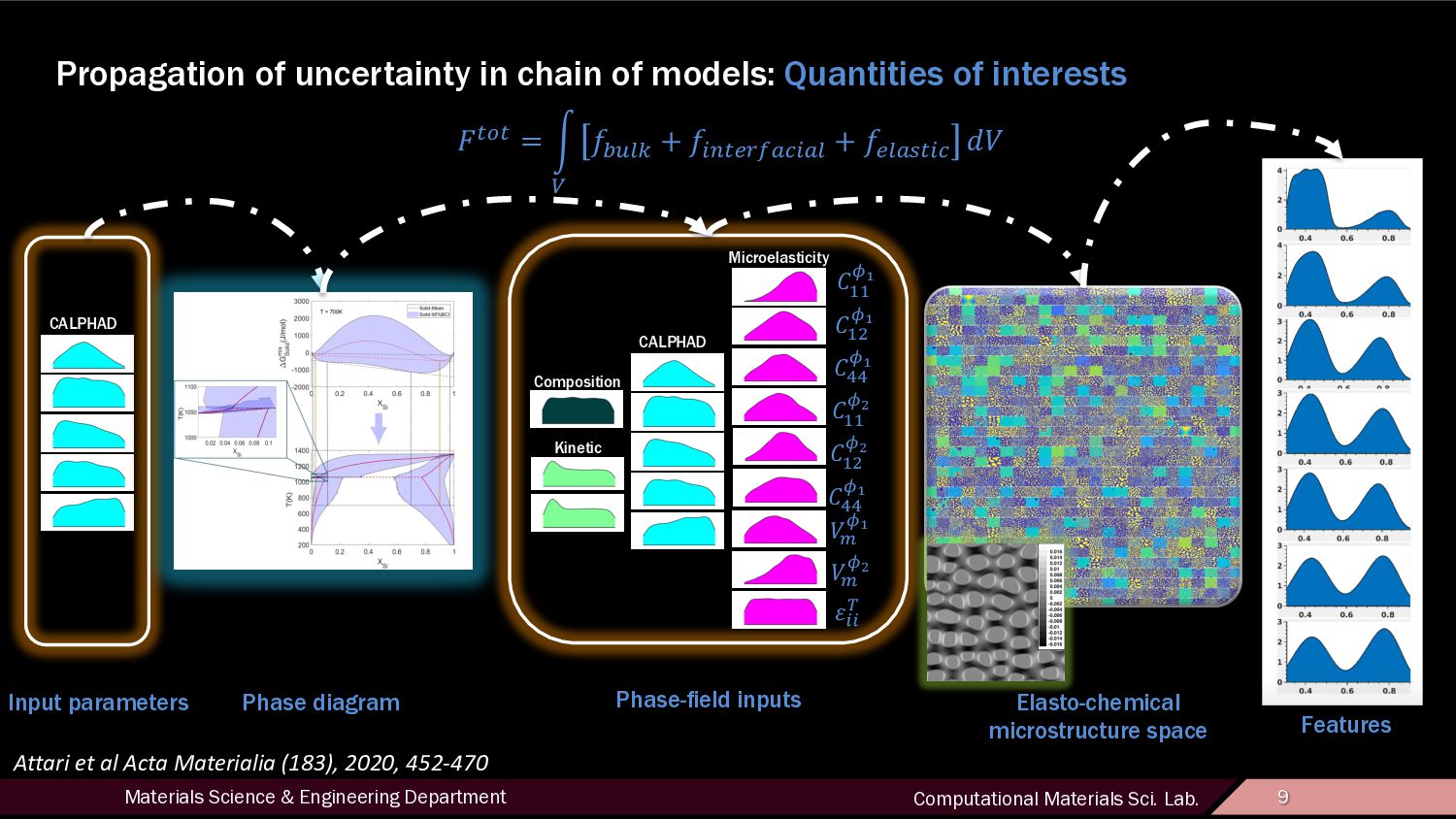
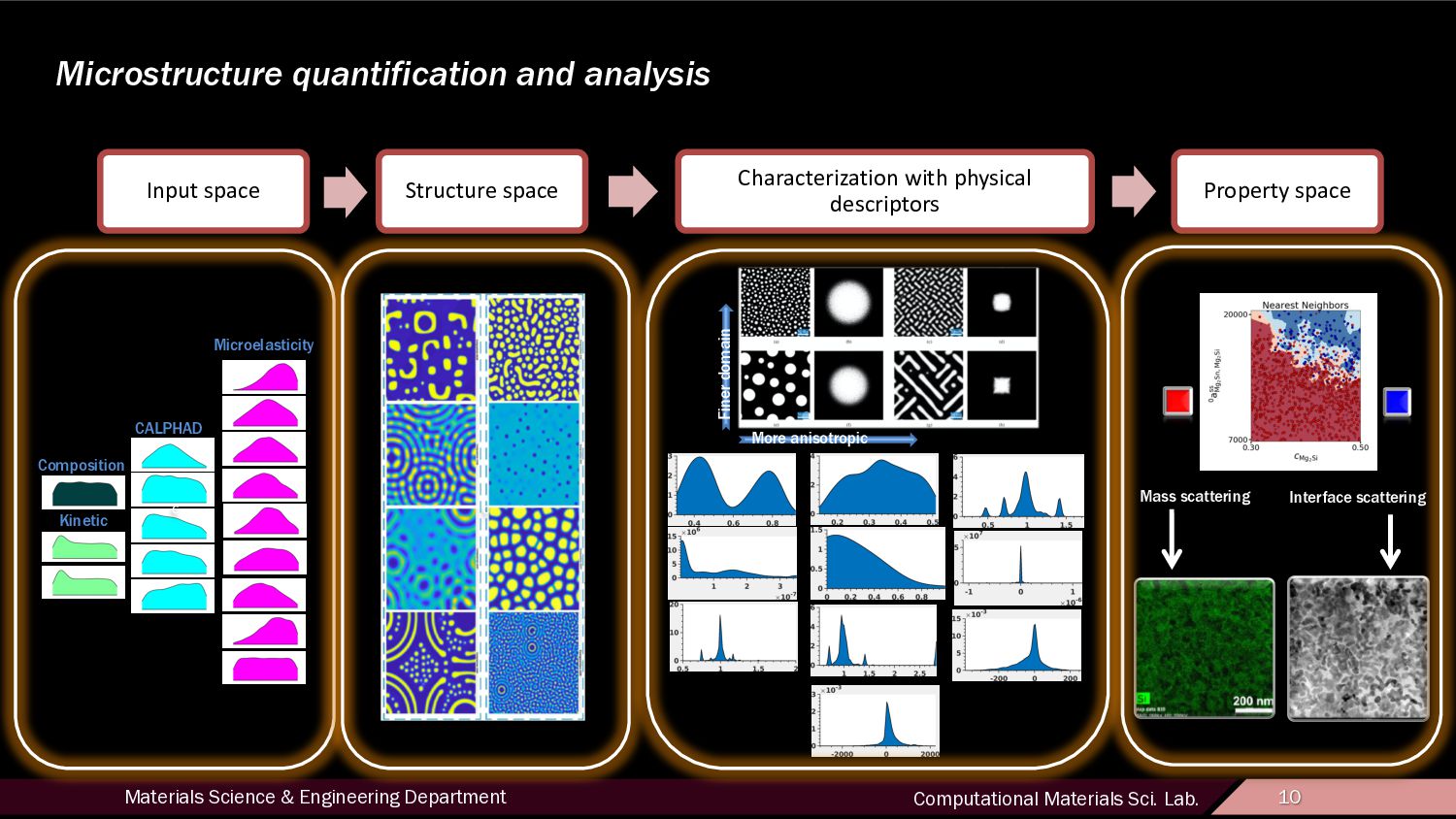
10 Input space Structure space Characterization with physical descriptors Property space Microstructure quantification and analysis Microelasticity Composition Kinetic CALPHAD c c Mass scattering Interface scattering More anisotropic Finer domain
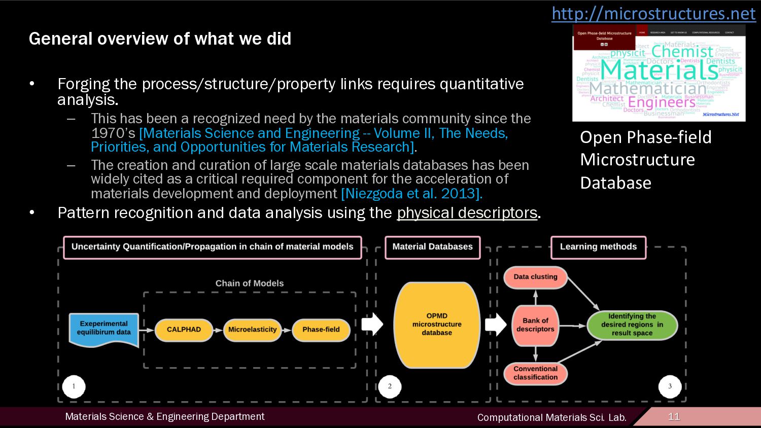
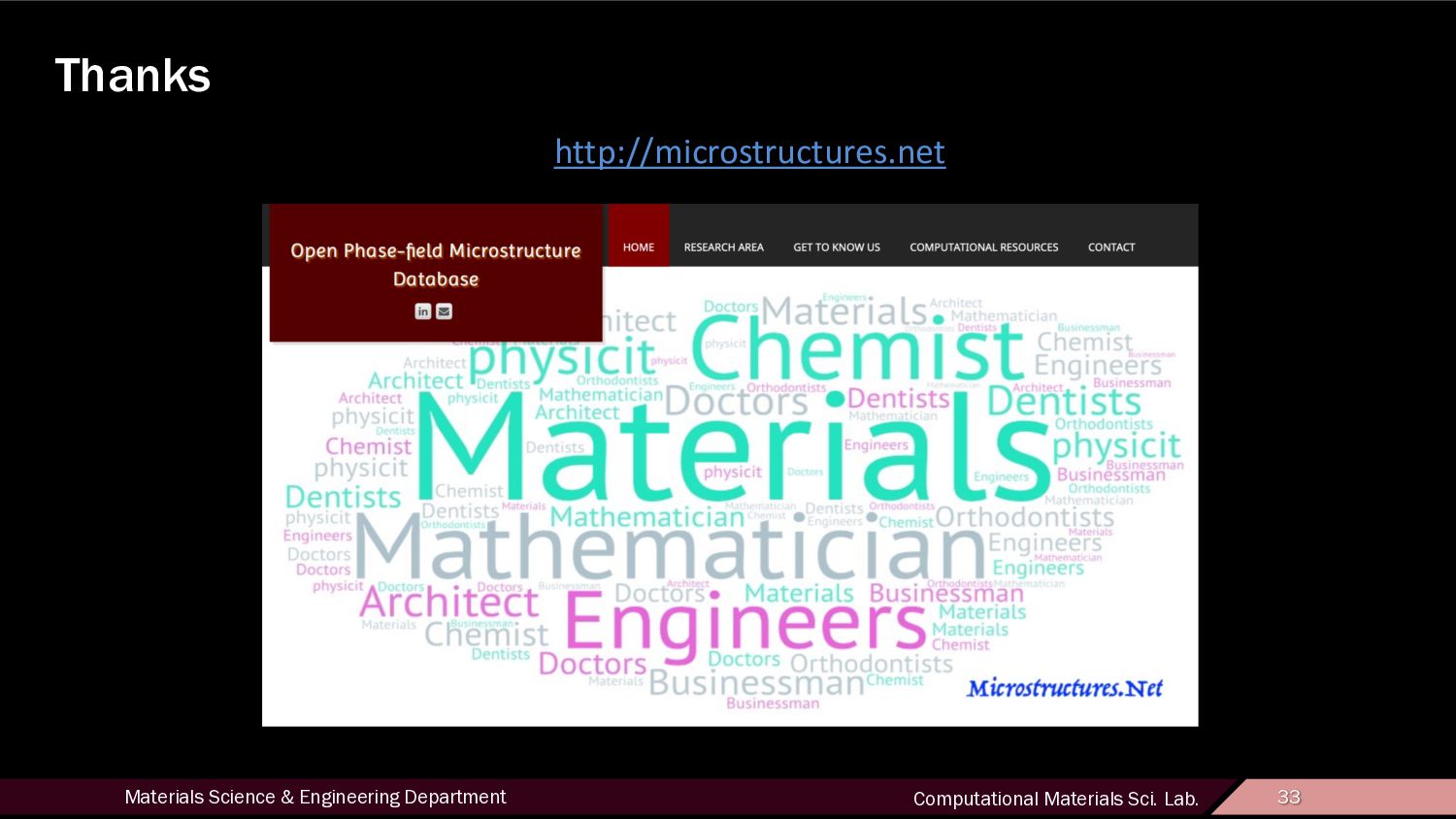
11 General overview of what we did • Forging the process/structure/property links requires quantitative analysis. – This has been a recognized need by the materials community since the 1970’s [Materials Science and Engineering -- Volume II, The Needs, Priorities, and Opportunities for Materials Research]. – The creation and curation of large scale materials databases has been widely cited as a critical required component for the acceleration of materials development and deployment [Niezgoda et al. 2013]. • Pattern recognition and data analysis using the physical descriptors. http://microstructures.net Open Phase-field Microstructure Database
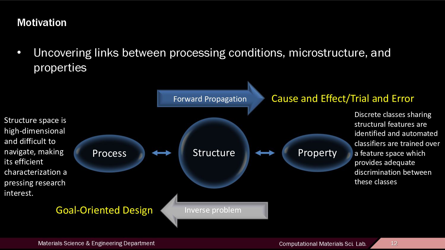
12 Motivation • Uncovering links between processing conditions, microstructure, and properties Process Structure Property Forward Propagation Inverse problem Cause and Effect/Trial and Error Goal-Oriented Design Structure space is high-dimensional and difficult to navigate, making its efficient characterization a pressing research interest. Discrete classes sharing structural features are identified and automated classifiers are trained over a feature space which provides adequate discrimination between these classes
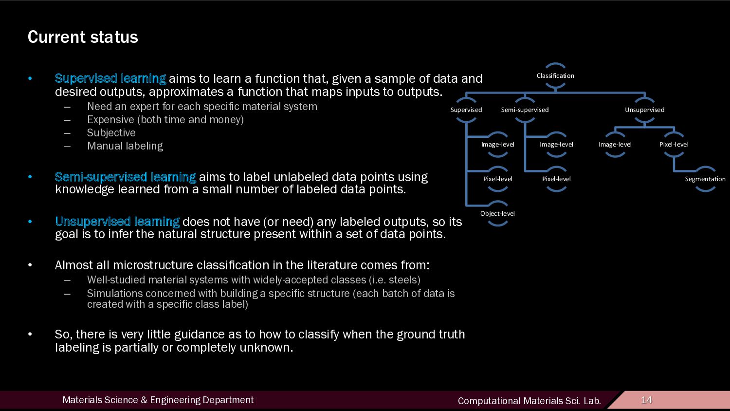
14 Current status • Supervised learning aims to learn a function that, given a sample of data and desired outputs, approximates a function that maps inputs to outputs. – Need an expert for each specific material system – Expensive (both time and money) – Subjective – Manual labeling • Semi-supervised learning aims to label unlabeled data points using knowledge learned from a small number of labeled data points. • Unsupervised learning does not have (or need) any labeled outputs, so its goal is to infer the natural structure present within a set of data points. • Almost all microstructure classification in the literature comes from: – Well-studied material systems with widely-accepted classes (i.e. steels) – Simulations concerned with building a specific structure (each batch of data is created with a specific class label) • So, there is very little guidance as to how to classify when the ground truth labeling is partially or completely unknown. Classification Supervised Image-level Pixel-level Object-level Semi-supervised Image-level Pixel-level Unsupervised Image-level Pixel-level Segmentation
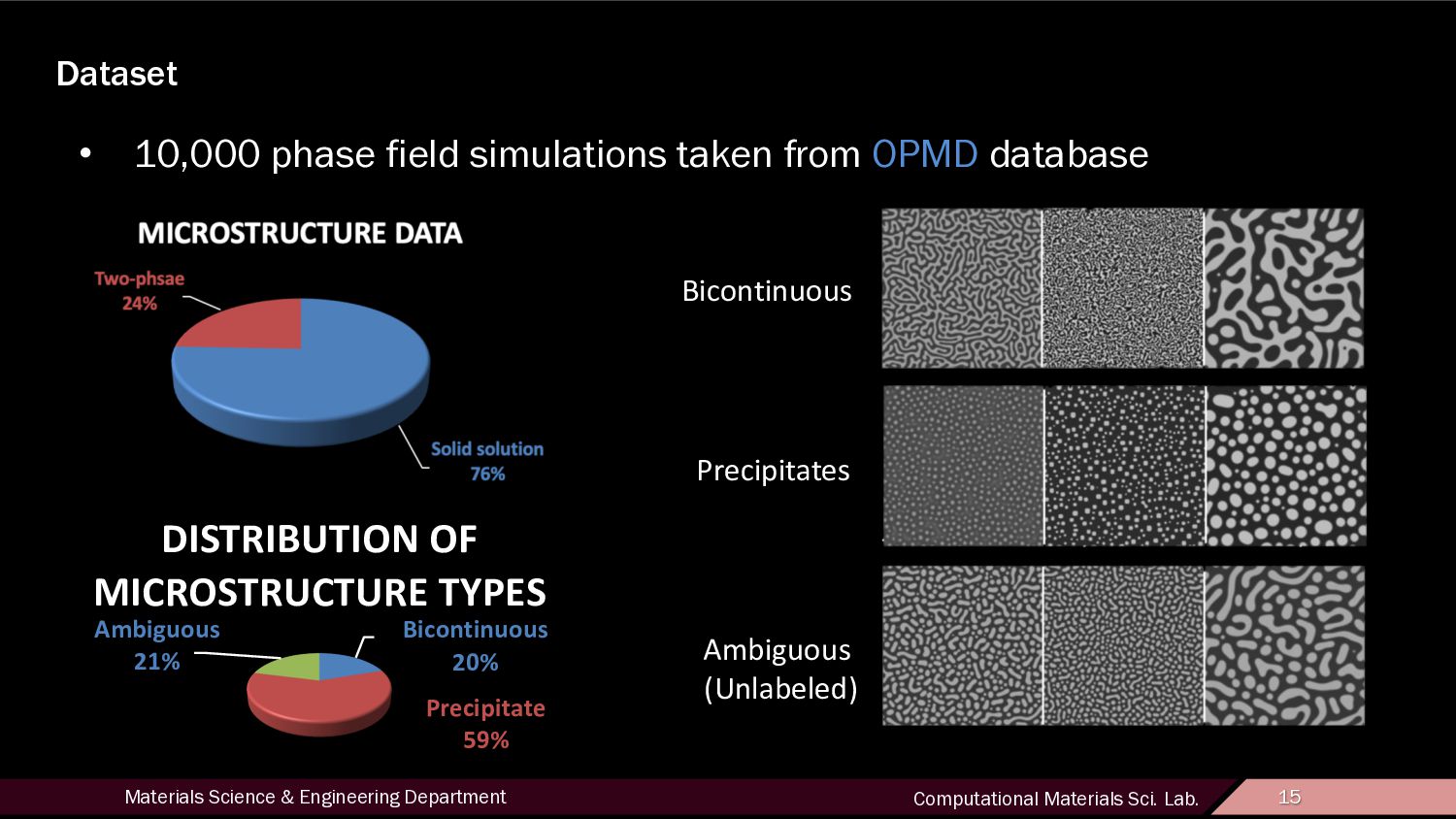
15 Dataset • 10,000 phase field simulations taken from OPMD database Bicontinuous 20% Precipitate 59% Ambiguous 21% DISTRIBUTION OF MICROSTRUCTURE TYPES Bicontinuous Precipitates Ambiguous (Unlabeled)
16 Image Processing • Binarization through the Otsu Method – Iterates through all possible thresholds and chooses the one where the sum of background and foreground variances is at a minimum The raw image Binarized version Black autocorrelation function
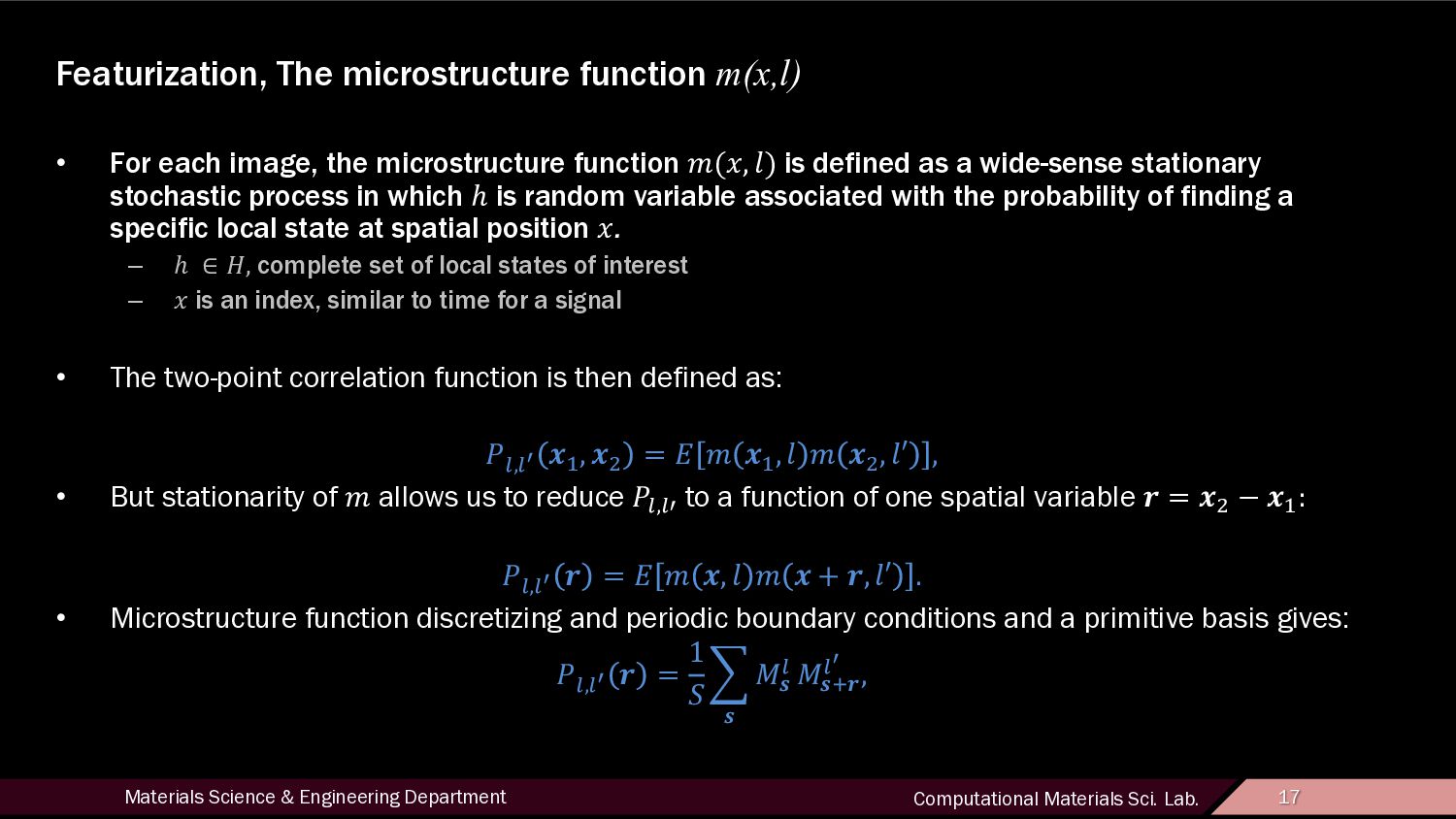
17 Featurization, The microstructure function m(x,l) • For each image, the microstructure function !(#, %) is defined as a wide-sense stationary stochastic process in which ℎ is random variable associated with the probability of finding a specific local state at spatial position #. – ℎ ∈ ), complete set of local states of interest – # is an index, similar to time for a signal • The two-point correlation function is then defined as: *+,+, -. , -/ = 1 ! -. , % ! -/ , %′ , • But stationarity of ! allows us to reduce *+,+3 to a function of one spatial variable 4 = -/ − -. : *+,+, 4 = 1 ! -, % ! - + 4, %′ . • Microstructure function discretizing and periodic boundary conditions and a primitive basis gives: *+,+, 4 = 1 : ; < =< + =<>4 +, ,
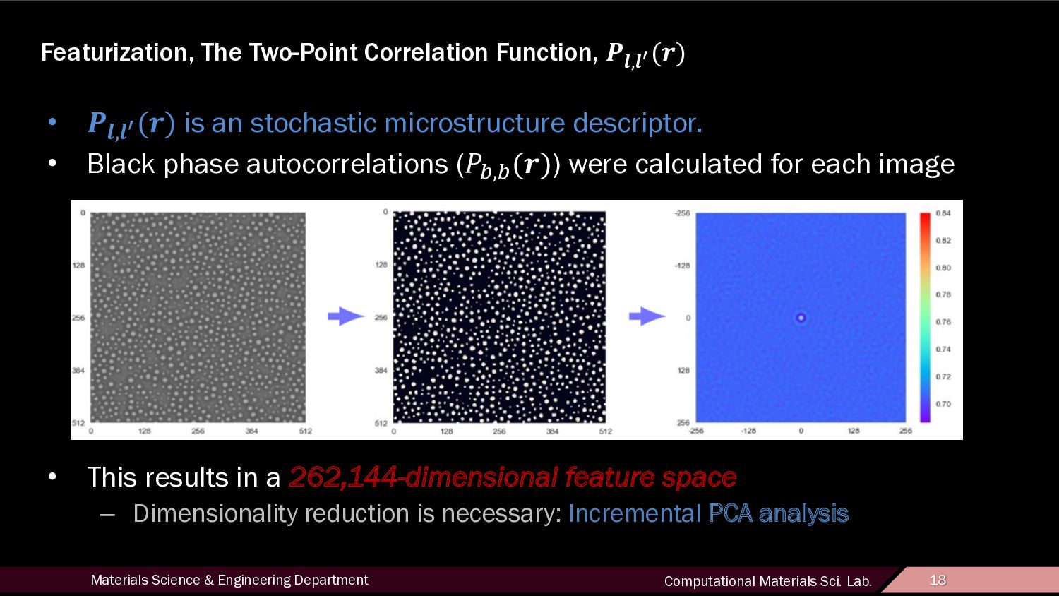
18 Featurization, The Two-Point Correlation Function, ! ","$ (&) • !","$ (&) is an stochastic microstructure descriptor. • Black phase autocorrelations ((),) (&)) were calculated for each image • This results in a 262,144-dimensional feature space – Dimensionality reduction is necessary: Incremental PCA analysis
19 Featurization Normalized Two-Point Correlation Function, !"##$,$&(#) • Why normalized? – Normalizing )*,* # removes the strong relationship with volume fraction, which allows a PCA decomposition of +,-- .,.& # to be used as a discriminative feature space based on structural information. • We define the normalized two-point correlation function as: +,-- .,.& # = 0 1 2, 3 1 2 + #, 35 − 0 1 2, 3 0[1 2 + #, 35 ] 9:-[1 2, 3 ] 9:-[1 2 + #, 35 ] . • For local state < at both endpoints, this reduces to: +,--*,* # = )*,* # − =* > =* − = * > where =* is the black phase volume fraction.
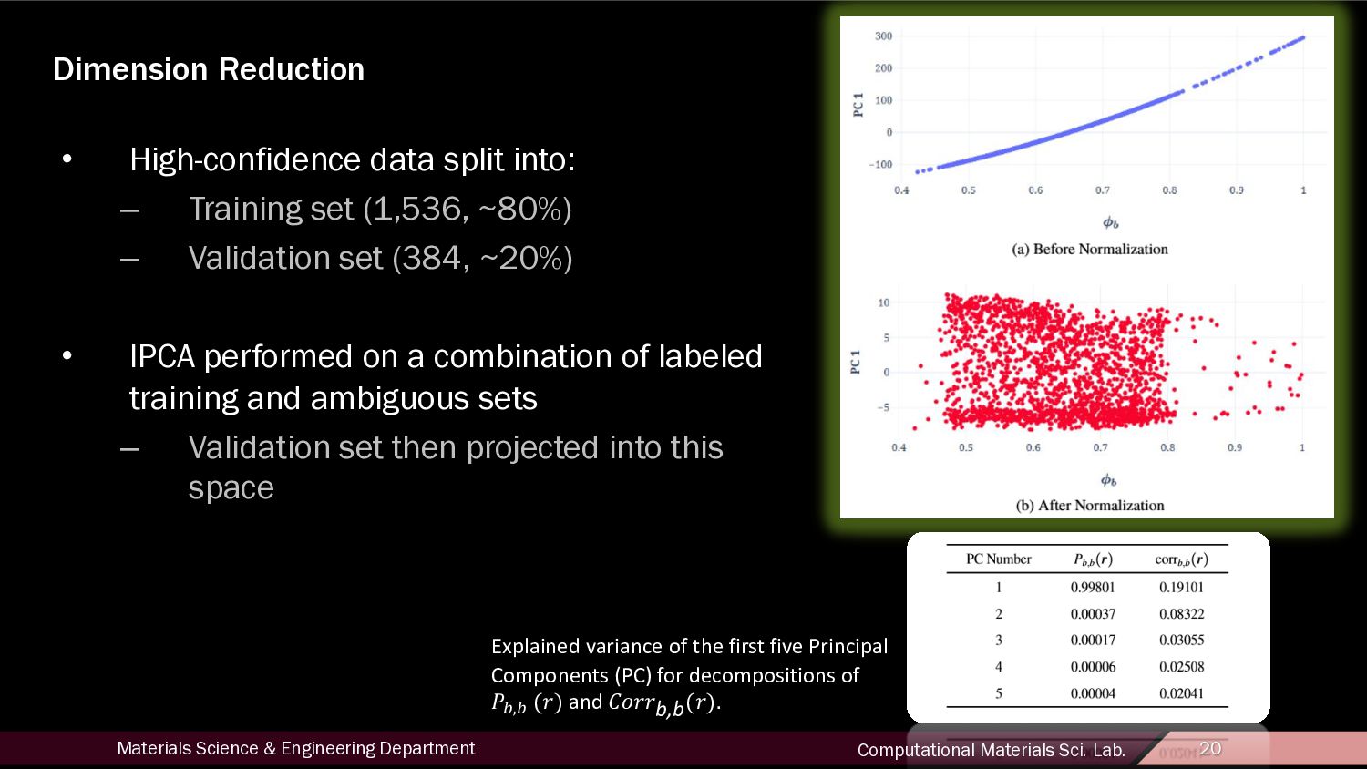
20 Dimension Reduction • High-confidence data split into: – Training set (1,536, ~80%) – Validation set (384, ~20%) • IPCA performed on a combination of labeled training and ambiguous sets – Validation set then projected into this space Explained variance of the first five Principal Components (PC) for decompositions of !"," (%) and '(%%b,b(%).
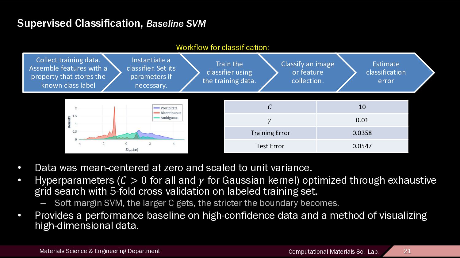
21 Supervised Classification, Baseline SVM • Data was mean-centered at zero and scaled to unit variance. • Hyperparameters (! > 0 for all and $ for Gaussian kernel) optimized through exhaustive grid search with 5-fold cross validation on labeled training set. – Soft margin SVM, the larger C gets, the stricter the boundary becomes. • Provides a performance baseline on high-confidence data and a method of visualizing high-dimensional data. ! 10 $ 0.01 Training Error 0.0358 Test Error 0.0547 Collect training data. Assemble features with a property that stores the known class label Instantiate a classifier. Set its parameters if necessary. Train the classifier using the training data. Classify an image or feature collection. Estimate classification error Workflow for classification:
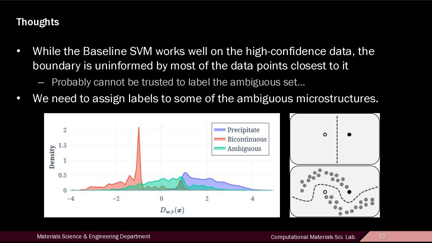
22 Thoughts • While the Baseline SVM works well on the high-confidence data, the boundary is uninformed by most of the data points closest to it – Probably cannot be trusted to label the ambiguous set… • We need to assign labels to some of the ambiguous microstructures.
23 Semi-Supervised Classification, Transductive SVMs • Uses both labeled and unlabeled data – Unlabeled data, when used in conjunction with a small amount of labeled data, can produce considerable improvement in learning accuracy. • There is always the danger that the wrong semi-supervised method will deteriorate classification performance instead of improving it – To alleviate this concern, a collection of methods with very different mathematical structures are used and the subset identified through their consensus is added to the training set • Supervised method modified to be semi-supervised • Now the problem is to find a boundary in the low density area of the labeled and unlabeled data while still maximizing training accuracy min 1 2 & ' + )* + ,-* . ξ, + )' + 0-* 1 2 ξ0 ∋ 4 50 ∈ −1,1 for < = 1, … , ? • Unfortunately, this problem is NP-hard – But, many methods have been proposed which approximate it
24 Semi-Supervised Classifiers • Method 1: Safe Semi-Supervised Support Vector Machine (S4VM), – Transductive SVM approximation algorithm which simultaneously considers multiple low-density separators instead of chasing one local minimum. • Method 2: Label Propagation (LP), – Graph-based method created for the semi-supervised problem • Method 3: COP-KMEANS Clustering (CKM), – Unsupervised method modified to be semi-supervised • Method 4: Modified Yarowsky Algorithm (MY), – Very popular self-training approach because it is easy to understand and can be a wrapper for any existing classifier. • Method 5: Updated training set,
26 Updated SVM • The four methods agreed on 301/519 of the initially unlabeled data (~58%) • This subset was added to the initially labeled training set, and an Updated SVM was optimized/trained over this set in the same fashion as the baseline Is there a significant difference? Classifier ! " Training Error (initially labeled) Test Error Baseline 10 0.01 0.0358 0.0547 Updated 10 0.01 0.0397 0.0599
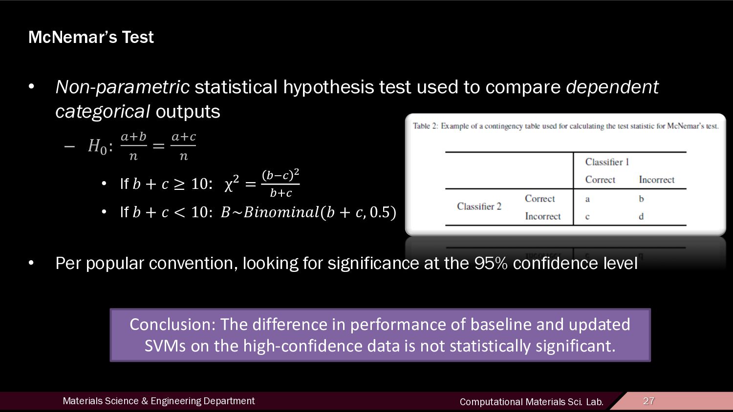
27 McNemar’s Test • Non-parametric statistical hypothesis test used to compare dependent categorical outputs – !" : $%& ' = $%) ' • If * + , ≥ 10: χ1 = &2) 3 &%) • If * + , < 10: 5~5789:78;<(* + ,, 0.5) • Per popular convention, looking for significance at the 95% confidence level Conclusion: The difference in performance of baseline and updated SVMs on the high-confidence data is not statistically significant.
28 Semi-Supervised Error Estimation • Since there is a set of data for which we do not know the labels, we cannot use traditional error estimation techniques for model validation. A tedious derivation leads to the conclusion: ! = # $ ∈ &' !' + # $ ∈ &) !) ⇒ ̂ ! = , # $ ∈ &' ̂ !' + , # $ ∈ &) ̂ !) . • This means that we can get a semi-supervised error estimate through separate supervised and unsupervised error estimates (with probabilities estimated by total numbers of labeled and labeled sample points). • ̂ !) can be estimated through a traditional test set – but what about ̂ !'? • Labeled subpopulation &) • Unlabeled subpopulation &'
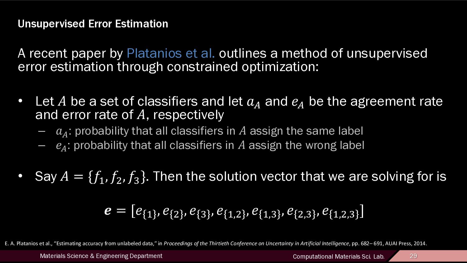
29 Unsupervised Error Estimation A recent paper by Platanios et al. outlines a method of unsupervised error estimation through constrained optimization: • Let ! be a set of classifiers and let "# and $# be the agreement rate and error rate of !, respectively – "#: probability that all classifiers in ! assign the same label – $#: probability that all classifiers in ! assign the wrong label • Say ! = {'( , '* , '+ }. Then the solution vector that we are solving for is - = [$ ( , $ * , $ + , $ (,* , $ (,+ , $ *,+ , $ (,*,+ ] E. A. Platanios et al., “Estimating accuracy from unlabeled data,” in Proceedings of the Thirtieth Conference on Uncertainty in Artificial Intelligence, pp. 682– 691, AUAI Press, 2014.
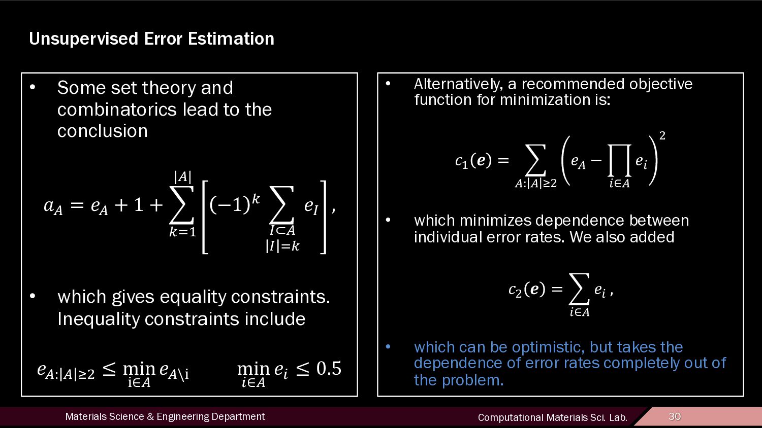
30 Unsupervised Error Estimation • Some set theory and combinatorics lead to the conclusion !" = $" + 1 + ' ()* |"| −1 ( ' -⊂" - )( $- , • which gives equality constraints. Inequality constraints include $": " 12 ≤ min 7∈" $"\7 min :∈" $: ≤ 0.5 • Alternatively, a recommended objective function for minimization is: >* ? = ' ": " 12 $" − @ :∈" $: 2 • which minimizes dependence between individual error rates. We also added >2 ? = ' :∈" $: , • which can be optimistic, but takes the dependence of error rates completely out of the problem.
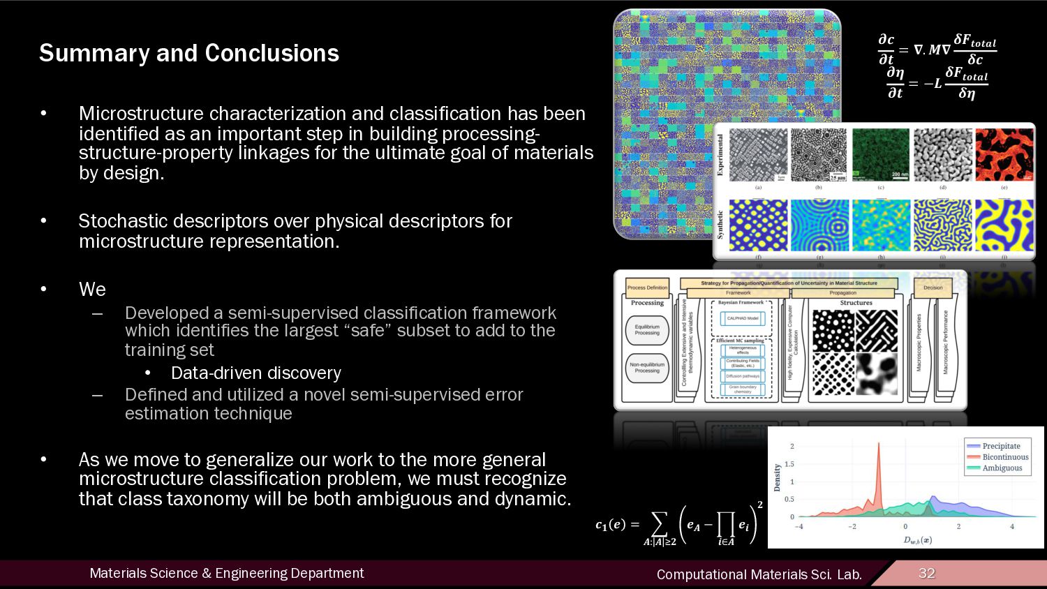
32 Summary and Conclusions • Microstructure characterization and classification has been identified as an important step in building processing- structure-property linkages for the ultimate goal of materials by design. • Stochastic descriptors over physical descriptors for microstructure representation. • We – Developed a semi-supervised classification framework which identifies the largest “safe” subset to add to the training set • Data-driven discovery – Defined and utilized a novel semi-supervised error estimation technique • As we move to generalize our work to the more general microstructure classification problem, we must recognize that class taxonomy will be both ambiguous and dynamic. !" # = % &: & () #& − + ,∈& #, ) .! ./ = 0. 20 34/5/67 3! .8 ./ = −9 34/5/67 38