SymPhas: Symbolic Algebra for Phase-Field Simulations

Transcript

1. SymPhas: Symbolic Algebra for Phase-Field Simulations Steven Silber Dr. Mikko Karttunen Western University, London, ON, Canada 1
2. Agenda 1. SymPhas 2. Problem Representation 3. Symbolic Algebra 4. Simulation Examples 2 S. A. Silber and M. Karttunen, “SymPhas —General Purpose Software for Phase- Field, Phase-Field Crystal, and Reaction- Diffusion Simulations,” Adv. Theory Simul., vol. 5, Art. no. 1, Dec. 2021.
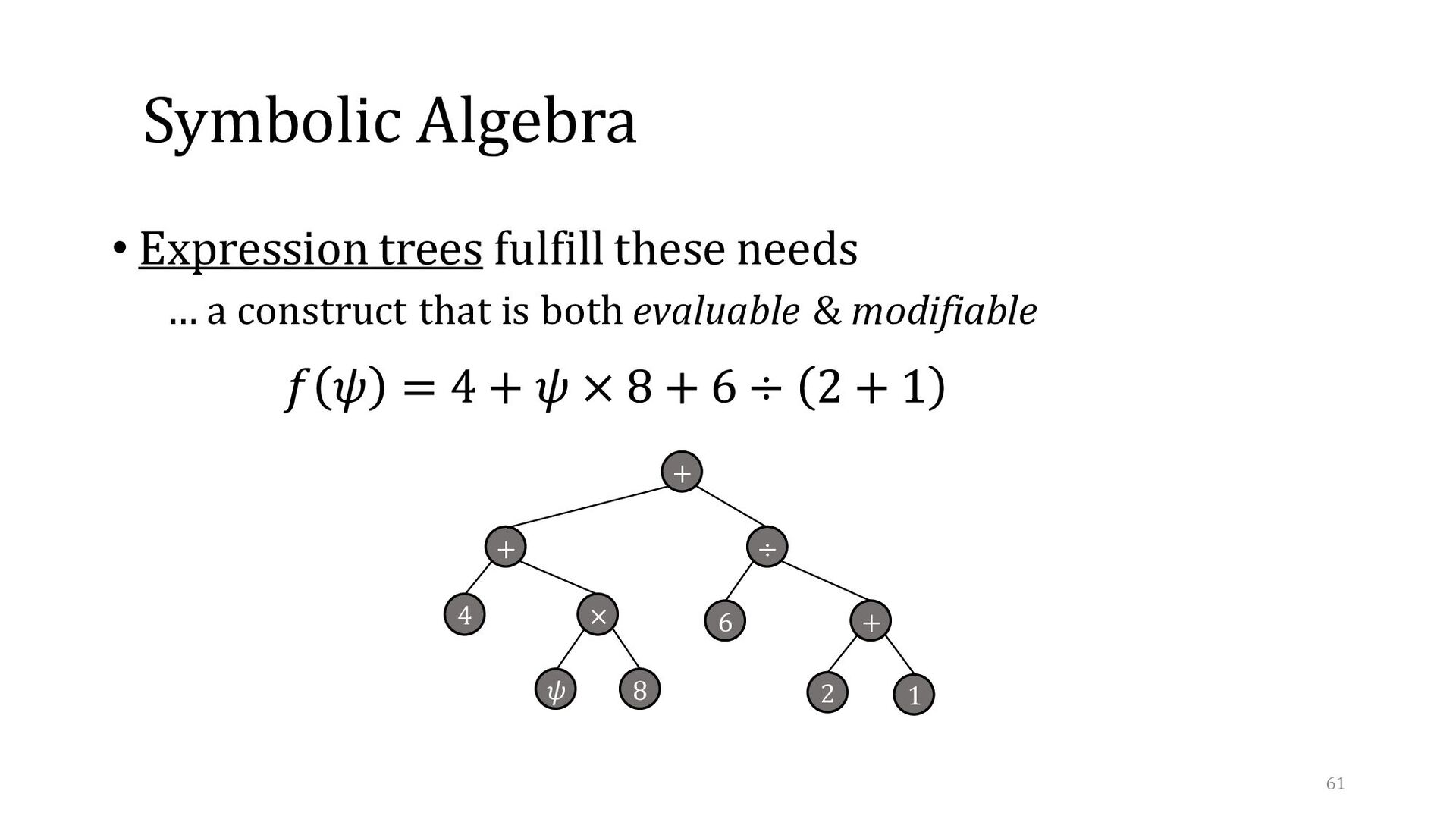
3. What is SymPhas? • C++ API & software • Numerical solutions to phase-field problems • P.F. Model → system of PDEs (1st order in time) • Symbolic algebra manipulation of phase-field models • User-defined P.F. Model → solver-enabled representation 3
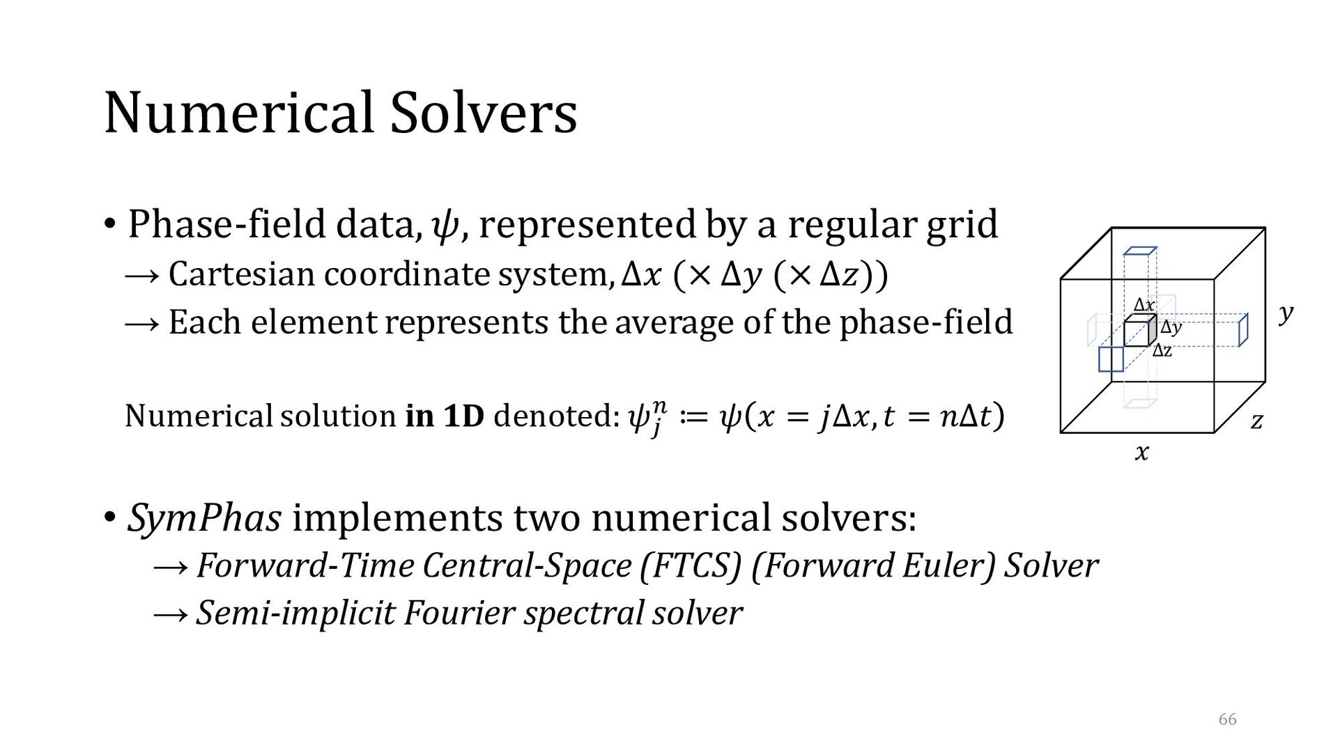
4. What is SymPhas? • Phase-field problems: • 1, 2, or 3 dimensions • Any number of order parameters • Real-, complex- or vector- valued order parameters • Phase-field, phase-field crystal or reaction-diffusion • I.e. User-defined P.F. Models 4
5. Objectives of SymPhas • Accessible • …to non-developers & those unfamiliar with C++ E.g. easy-to-use API + extensive documentation (Doxygen) • Efficient/high performance • Parallelization: Single-CPU • Efficient code design 5
6. Objectives of SymPhas 1. Unconstrained definition of phase-field models 2. Comprehensive symbolic algebra functionality 3. Modular numerical solvers 6
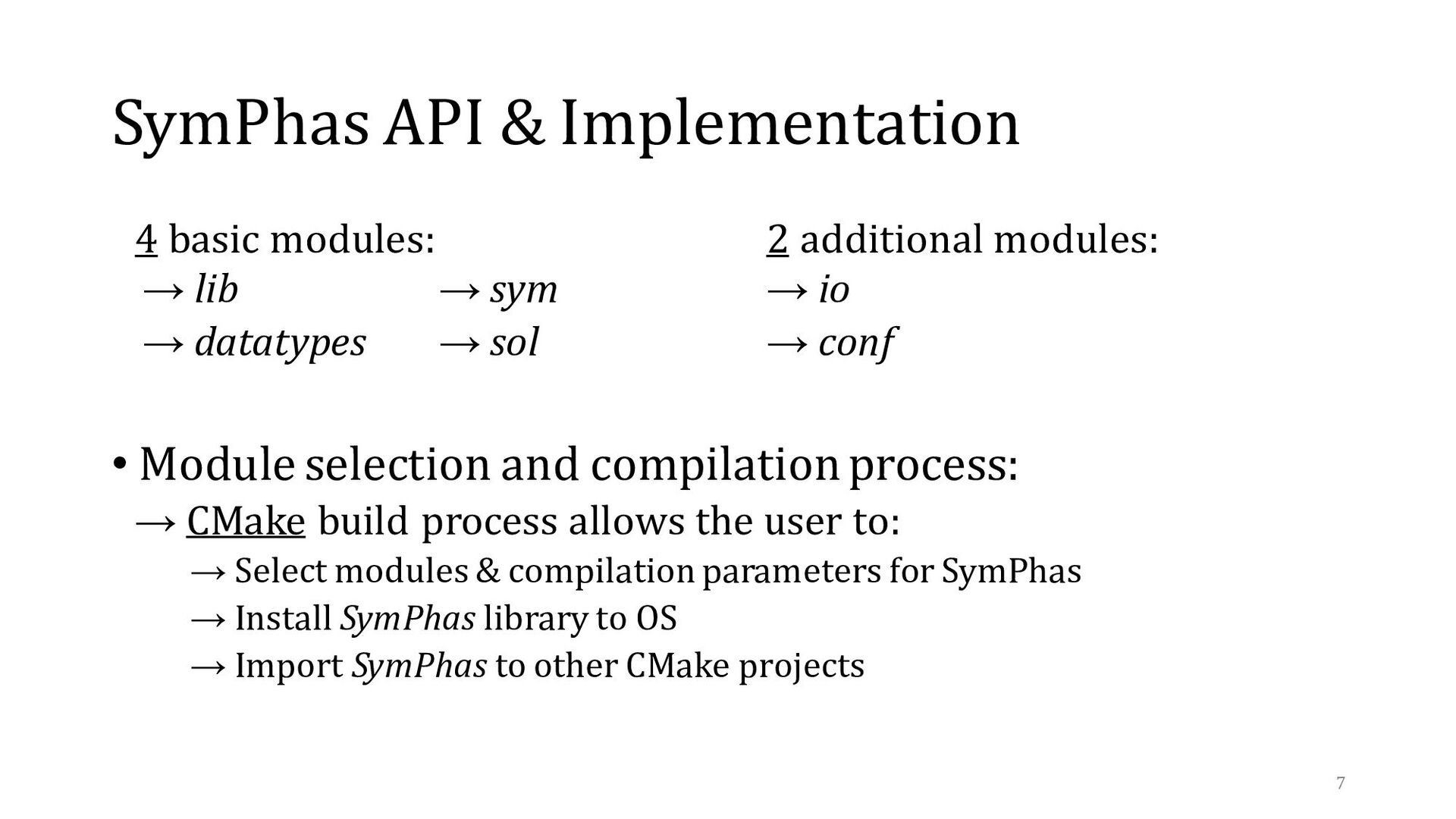
7. 4 basic modules: 2 additional modules: → lib → sym → io → datatypes → sol → conf • Module selection and compilation process: → CMake build process allows the user to: → Select modules & compilation parameters for SymPhas → Install SymPhas library to OS → Import SymPhas to other CMake projects SymPhas API & Implementation 7
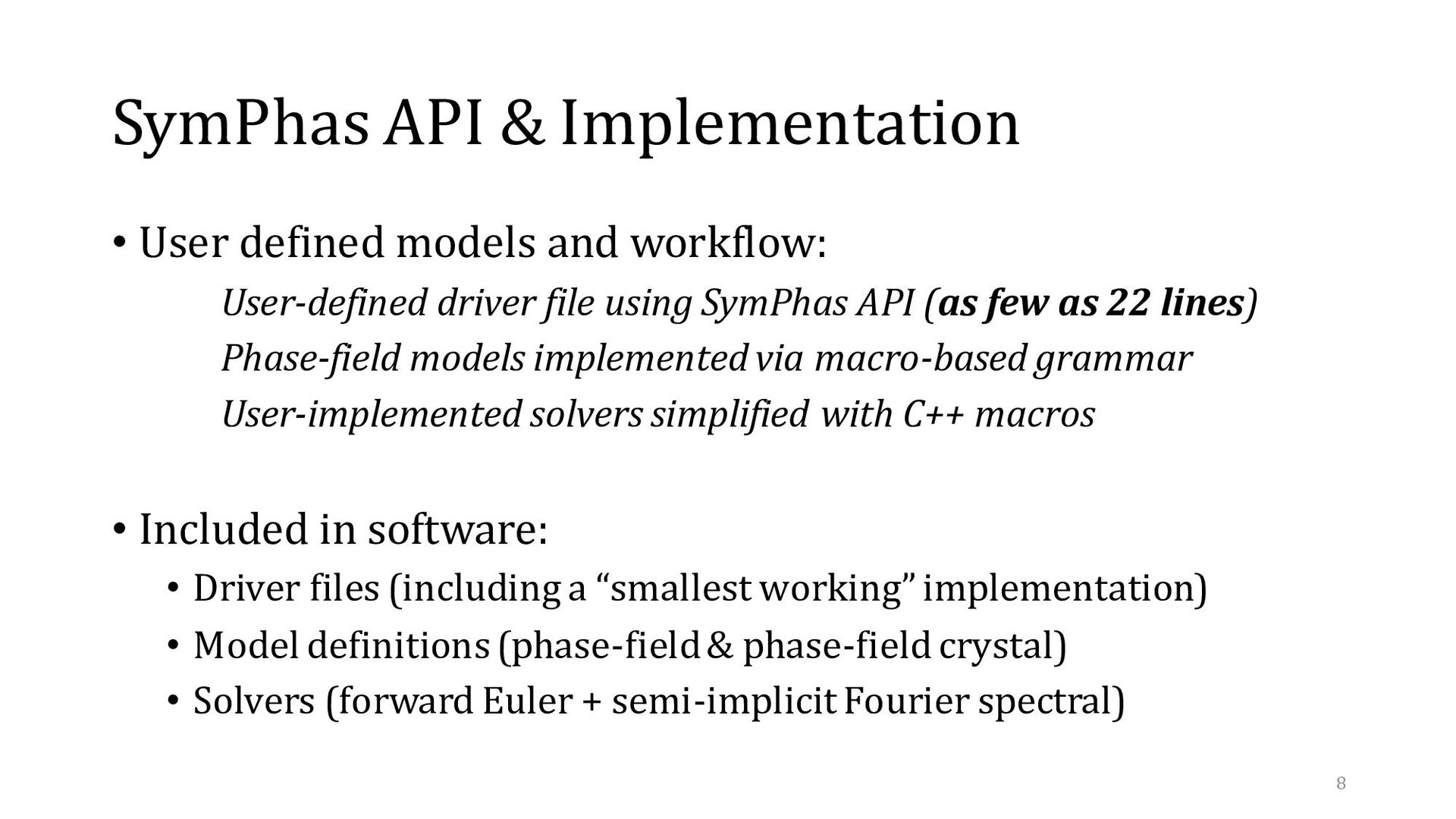
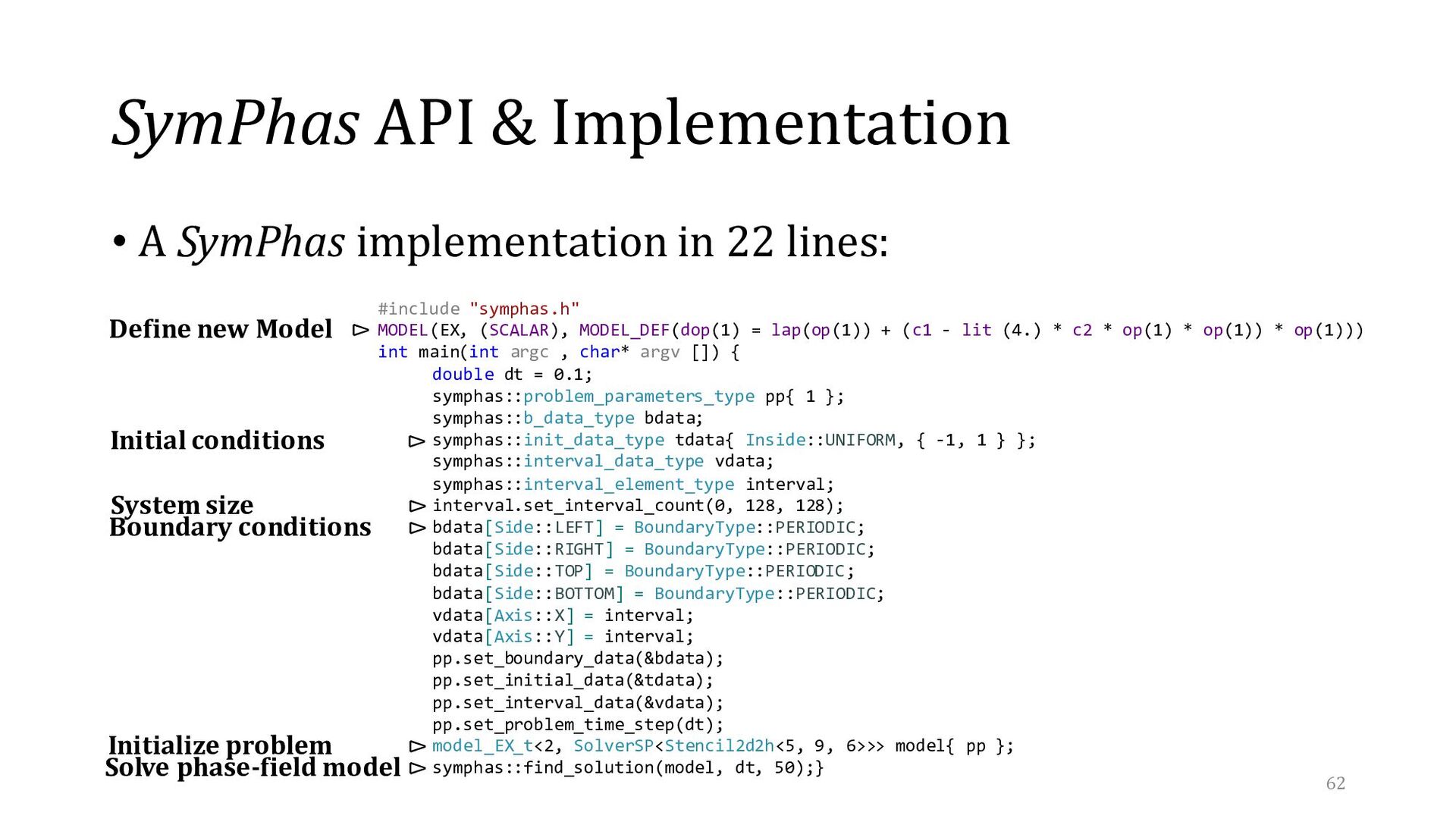
8. SymPhas API & Implementation • User defined models and workflow: User-defined driver file using SymPhas API (as few as 22 lines) Phase-field models implemented via macro-based grammar User-implemented solvers simplified with C++ macros • Included in software: • Driver files (including a “smallest working” implementation) • Model definitions (phase-field & phase-field crystal) • Solvers (forward Euler + semi-implicit Fourier spectral) 8
9. SymPhas API & Implementation • Design with best practises and maintenance-friendly techniques → Reducing coupling/increasing cohesion → Single responsibility principle → Common namespaces → Informative function names → Data groups → API specific type aliases + Extensive documentation (using Doxygen) Object design User facing functionality 9
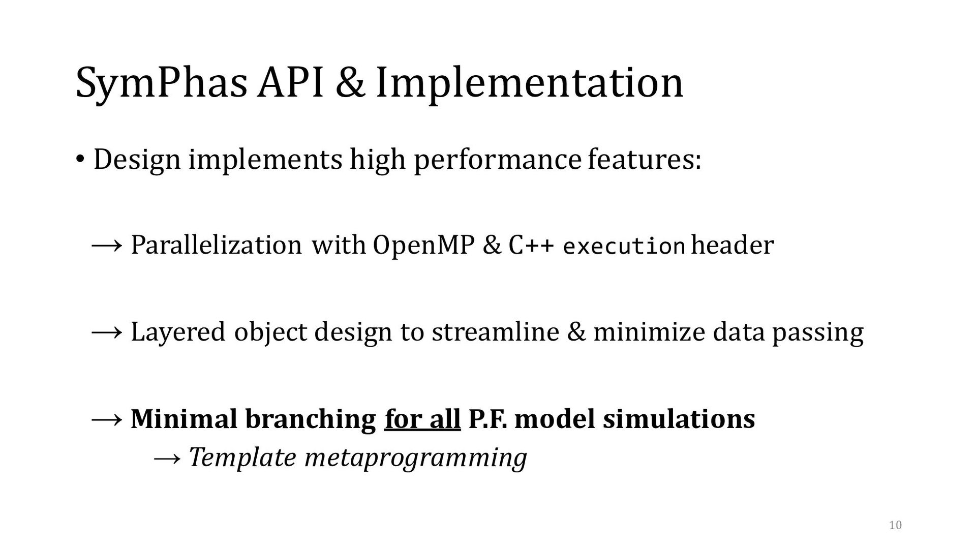
10. SymPhas API & Implementation • Design implements high performance features: → Parallelization with OpenMP & C++ execution header → Layered object design to streamline & minimize data passing → Minimal branching for all P.F. model simulations → Template metaprogramming 10
11. 2 | Problem Encapsulation 11
12. Problem Representation • C++ → Object Oriented Programming (OOP) • Generic programming AKA template metaprogramming → Everything is a type …As opposed to inheritance and virtual dispatch → C++ templates and generics → “Template argument deduction” 12
13. Problem Representation Uniform Grid Uniform Grid Uniform Grid 13
14. Problem Representation System Uniform Grid System Uniform Grid System Uniform Grid 14
15. Group of Systems Problem Representation System Uniform Grid System Uniform Grid System Uniform Grid 15
16. Group of Systems Problem Representation System Uniform Grid System Uniform Grid System Uniform Grid Equation of Motion Equation of Motion Equation of Motion 16
17. Group of Systems Problem Representation System Uniform Grid System Uniform Grid System Uniform Grid Equation of Motion Equation of Motion Equation of Motion 𝐸(𝜓1 , 𝜓2 , 𝜓3 ) 17
18. Group of Systems Problem Representation System Uniform Grid System Uniform Grid System Uniform Grid Equation of Motion Equation of Motion Equation of Motion 𝐸(𝜓1 , 𝜓2 , 𝜓3 ) 𝜓1 𝜓2 𝜓3 18
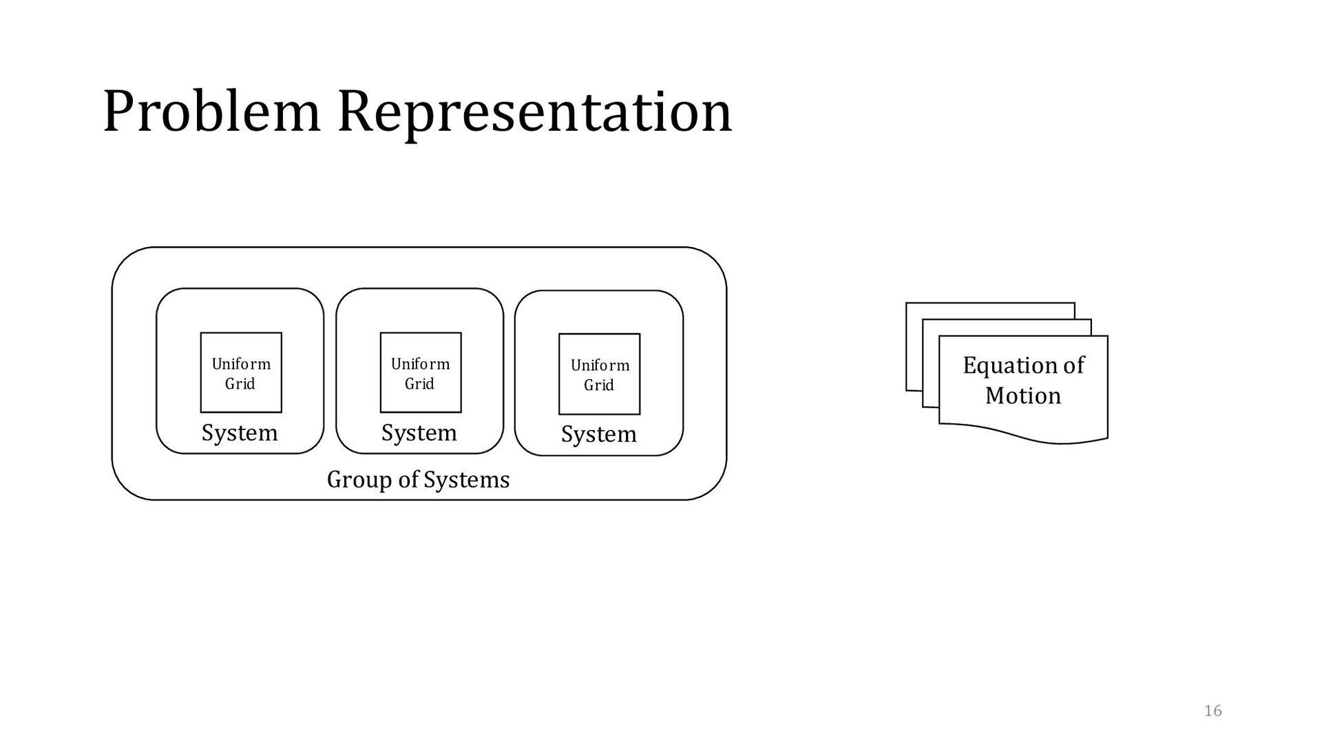
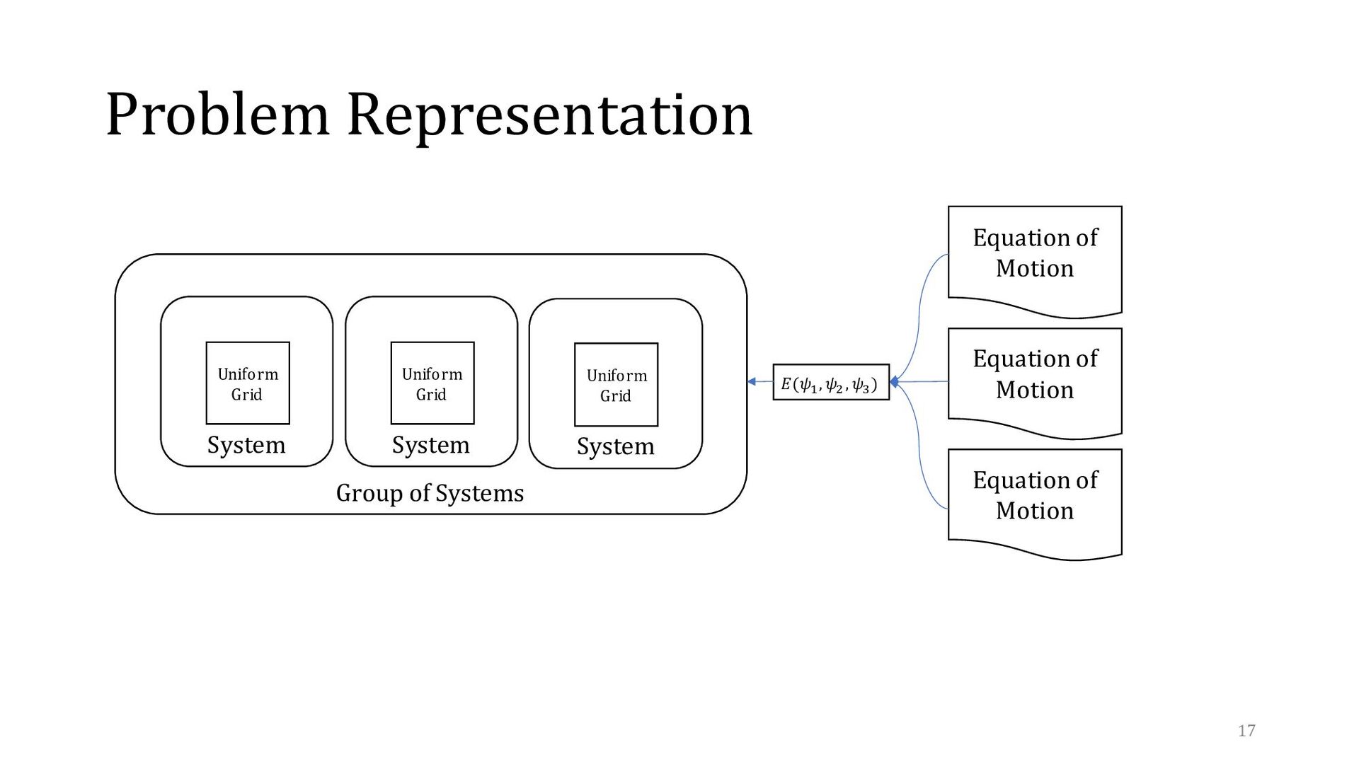
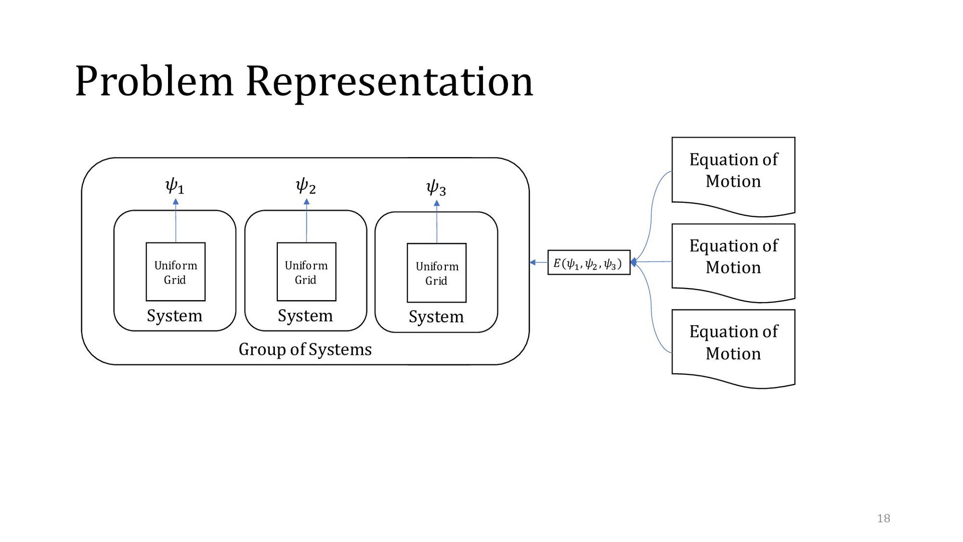
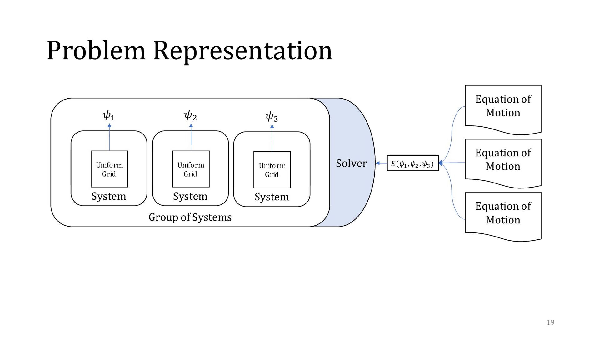
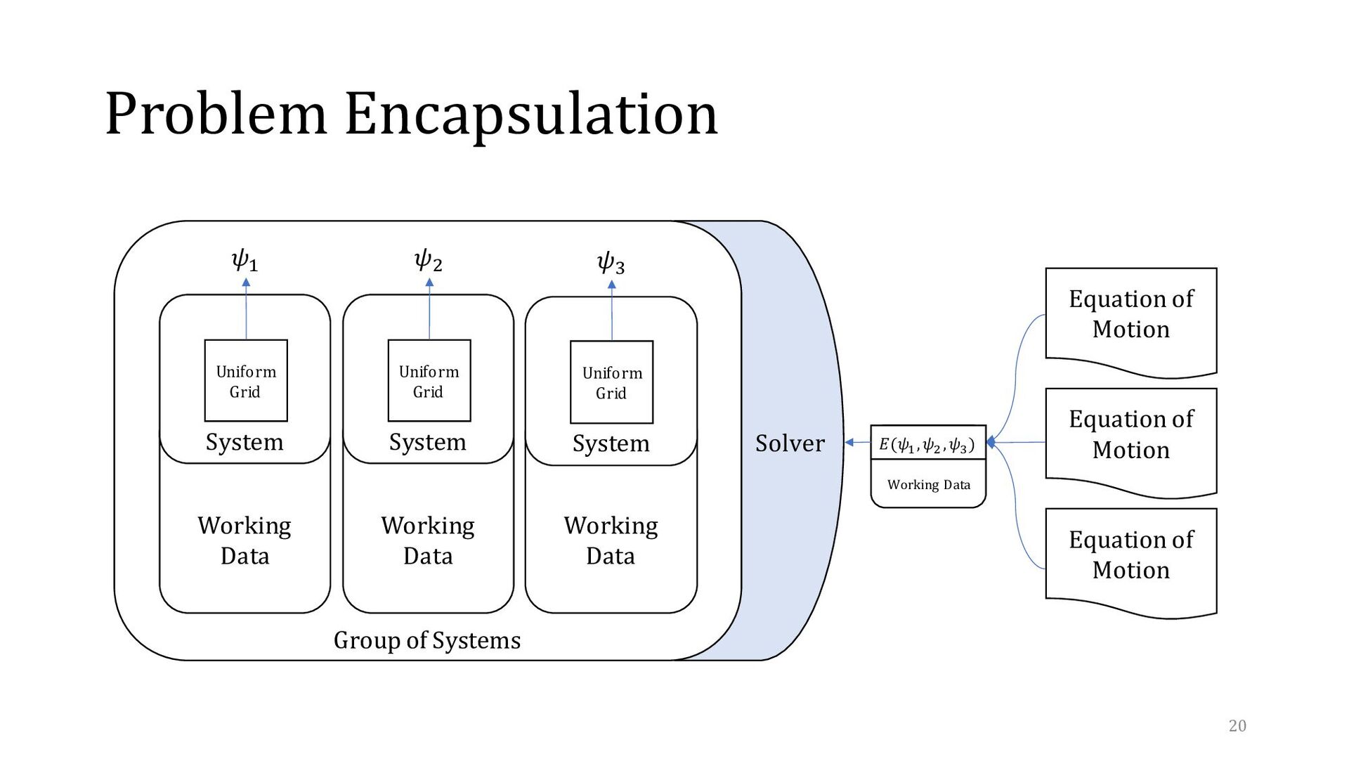
19. Working Data Group of Systems Problem Representation Working Data Working Data Working Data System System System Uniform Grid Uniform Grid Uniform Grid Equation of Motion Equation of Motion Equation of Motion 𝐸(𝜓1 , 𝜓2 , 𝜓3 ) 𝜓1 𝜓2 𝜓3 Solver 19
20. Working Data Group of Systems Problem Encapsulation Working Data Working Data Working Data System Uniform Grid System Uniform Grid System Uniform Grid Equation of Motion Equation of Motion Equation of Motion 𝐸(𝜓1 , 𝜓2 , 𝜓3 ) 𝜓1 𝜓2 𝜓3 Solver 20
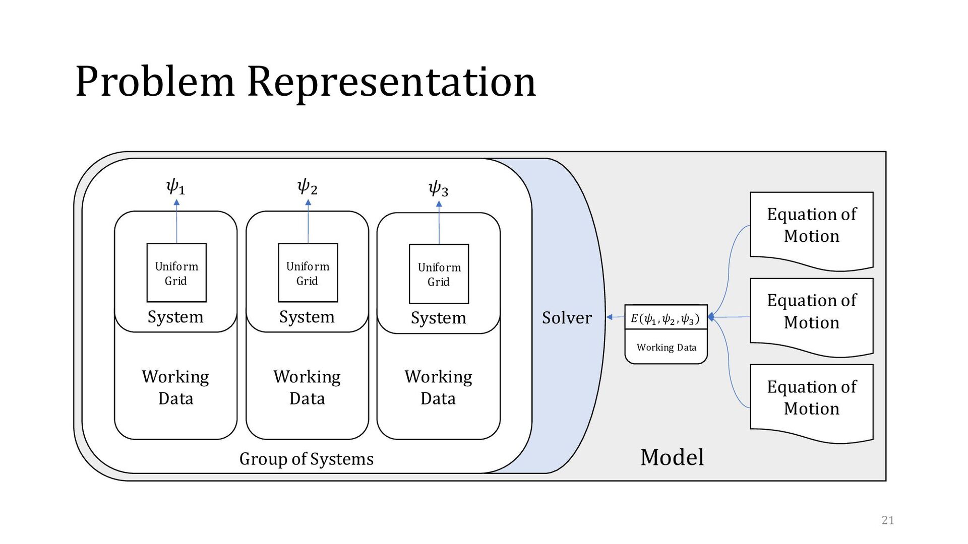
21. Model Group of Systems Problem Representation Working Data Working Data Working Data System Uniform Grid System Uniform Grid System Uniform Grid Equation of Motion Equation of Motion Working Data Equation of Motion 𝐸(𝜓1 , 𝜓2 , 𝜓3 ) 𝜓1 𝜓2 𝜓3 Solver 21
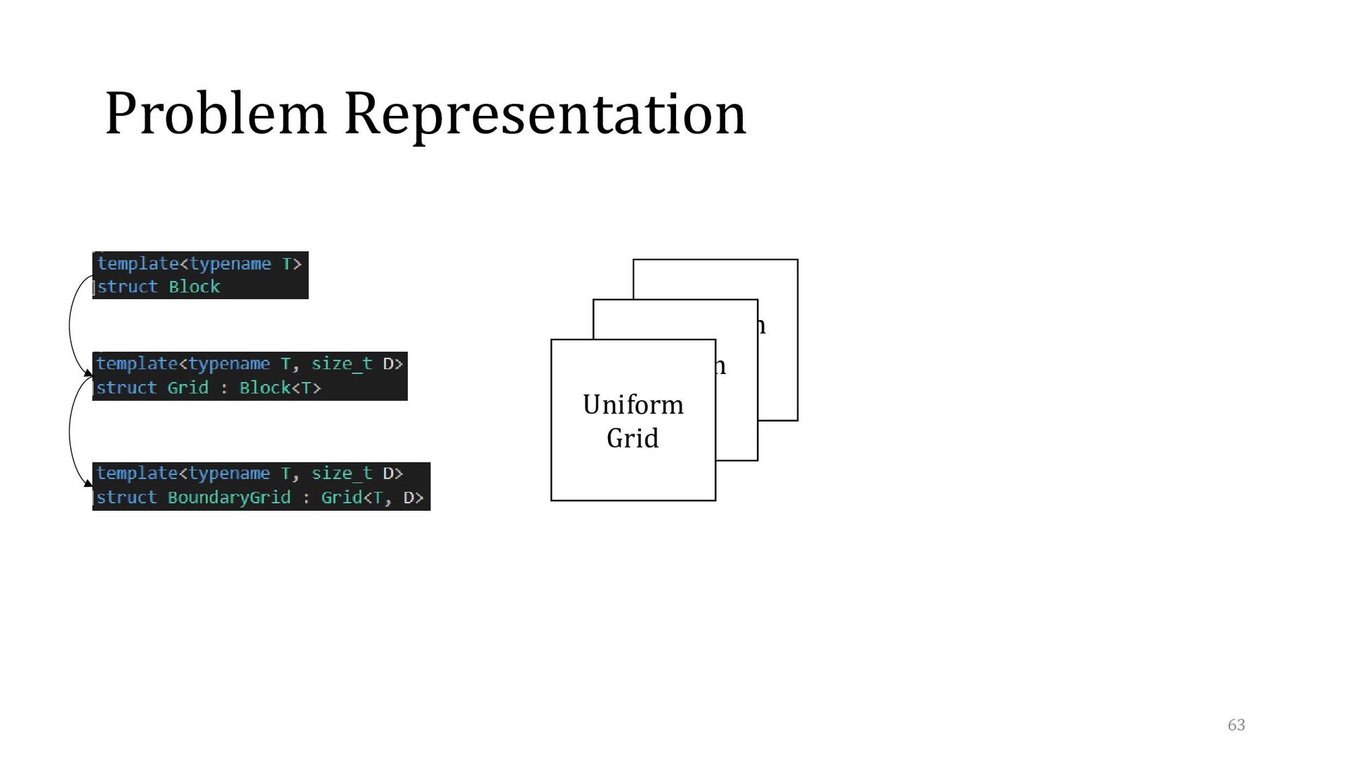
22. Problem Representation • OOP provides flexibility: • Different Solver implementations (incl. user-defined solvers) • Different System specializations based on Solver type • Different Grid specializations based on System type • Different Model types for phase-field and phase-field crystal problems 22
23. Problem Representation • User-defined phase-field models: 23 MODEL(GRAYSCOTT, (SCALAR, SCALAR), MODEL_DEF_PREAMBLE((auto prr = psi * rho * rho;), dpsi = c1 * lap(psi) - prr + c3 * (one - psi), drho = c2 * lap(rho) + prr - (c3 + c4) * rho) ) LINK_WITH_NAME(GRAYSCOTT, GRAYSCOTT) MODEL(MB, (SCALAR), MODEL_DEF( dpsi = -bilap(psi) - lap((c1 - c2 * psi * psi) * psi)) ) LINK_WITH_NAME(MB, MODELB) MODEL(MC, (SCALAR, SCALAR), MODEL_DEF_PREAMBLE( ( auto psi3 = psi * psi * psi; auto rho3 = rho * rho * rho; ), dpsi = lap(psi) + c1 * psi - c2 * psi3 + lit(2.) * c5 * psi * rho, drho = -bilap(rho) - lap(c3 * rho - c4 * rho3 + c5 * psi * psi)) ) LINK_WITH_NAME(MC, MODELC) DEFINE_MODEL_FIELD_NAMES(MC, ("psi", "m")) MODEL(MA, (SCALAR), MODEL_DEF( dpsi = lap(psi) + (c1 - c2 * psi * psi) * psi) ) LINK_WITH_NAME(MA, MODELA)
24. 3 | Symbolic Algebra 24
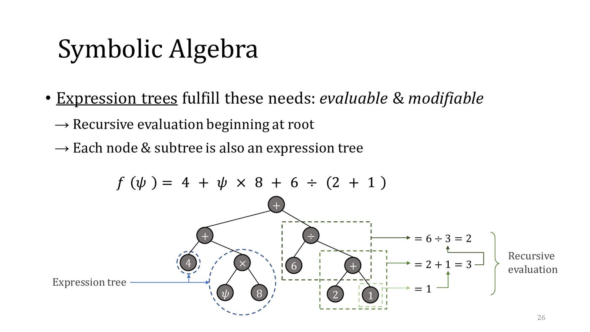
25. Symbolic Algebra • Representation of equation of motion? → Of the form… • How the equation will be used: → Evaluated multiple times (e.g., each solver loop) → Modified to fit the design of a given numerical solver 25
26. Symbolic Algebra Expression tree • Expression trees fulfill these needs: evaluable & modifiable → Recursive evaluation beginning at root → Each node & subtree is also an expression tree = 1 = 2 + 1 = 3 = 6 ÷ 3 = 2 Recursive evaluation + + 𝜓 8 × 4 1 2 ÷ 6 + 26
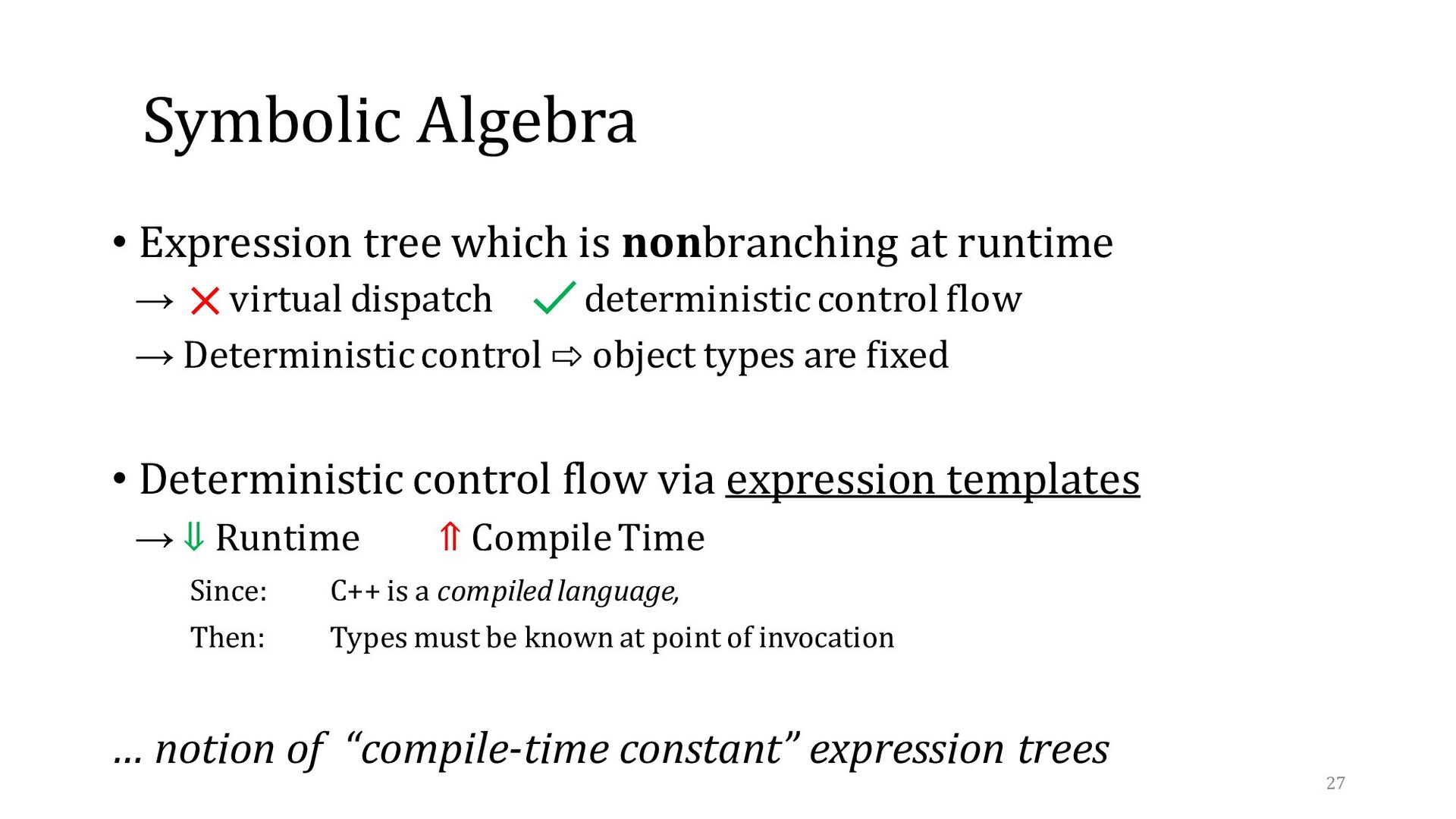
27. Symbolic Algebra • Expression tree which is nonbranching at runtime → virtual dispatch deterministic control flow → Deterministic control ⇨ object types are fixed • Deterministic control flow via expression templates → ⇓ Runtime ⇑ Compile Time Since: C++ is a compiled language, Then: Types must be known at point of invocation … notion of “compile-time constant” expression trees 27
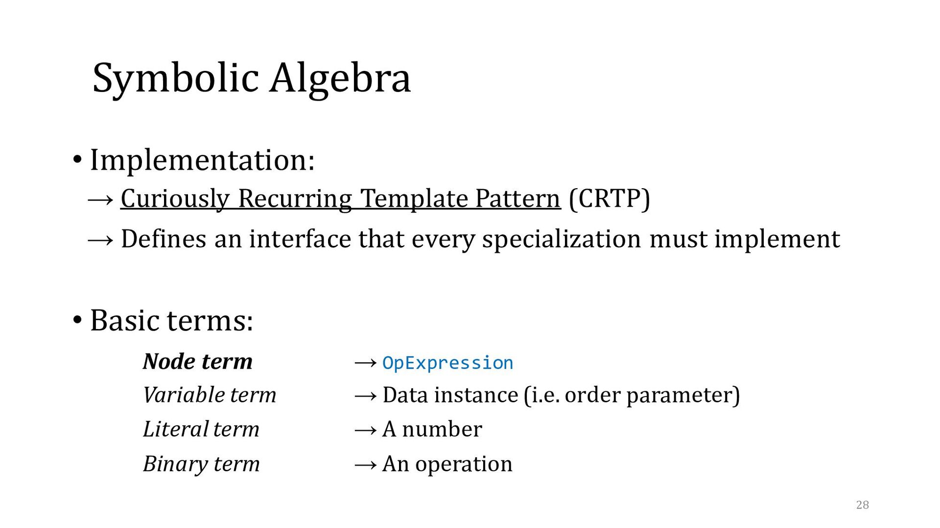
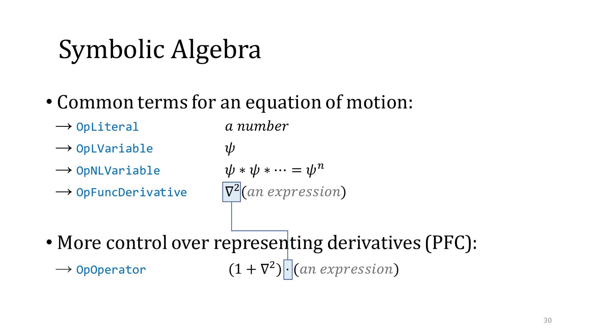
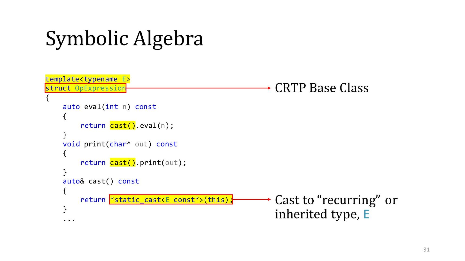
28. Symbolic Algebra • Implementation: → Curiously Recurring Template Pattern (CRTP) → Defines an interface that every specialization must implement • Basic terms: Node term → OpExpression Variable term → Data instance (i.e. order parameter) Literal term → A number Binary term → An operation 28
29. Symbolic Algebra • Binary Operators → OpBinaryAdd → OpBinarySub → OpBinaryMul → OpBinaryDiv • Implements operator overloads • Order of operations of overloaded operator is always followed 29
30. Symbolic Algebra • Common terms for an equation of motion: → OpLiteral 𝑎 𝑛𝑢𝑚𝑏𝑒𝑟 → OpLVariable 𝜓 → OpNLVariable 𝜓 ∗ 𝜓 ∗ ⋯ = 𝜓𝑛 → OpFuncDerivative ∇2(𝑎𝑛 𝑒𝑥𝑝𝑟𝑒𝑠𝑠𝑖𝑜𝑛) • More control over representing derivatives (PFC): → OpOperator (1 + ∇2) ⋅ (𝑎𝑛 𝑒𝑥𝑝𝑟𝑒𝑠𝑠𝑖𝑜𝑛) 30
31. Cast to “recurring” or inherited type, E template<typename E> struct OpExpression { auto eval(int n) const { return cast().eval(n); } void print(char* out) const { return cast().print(out); } auto& cast() const { return *static_cast<E const*>(this); } ... Symbolic Algebra CRTP Base Class 31
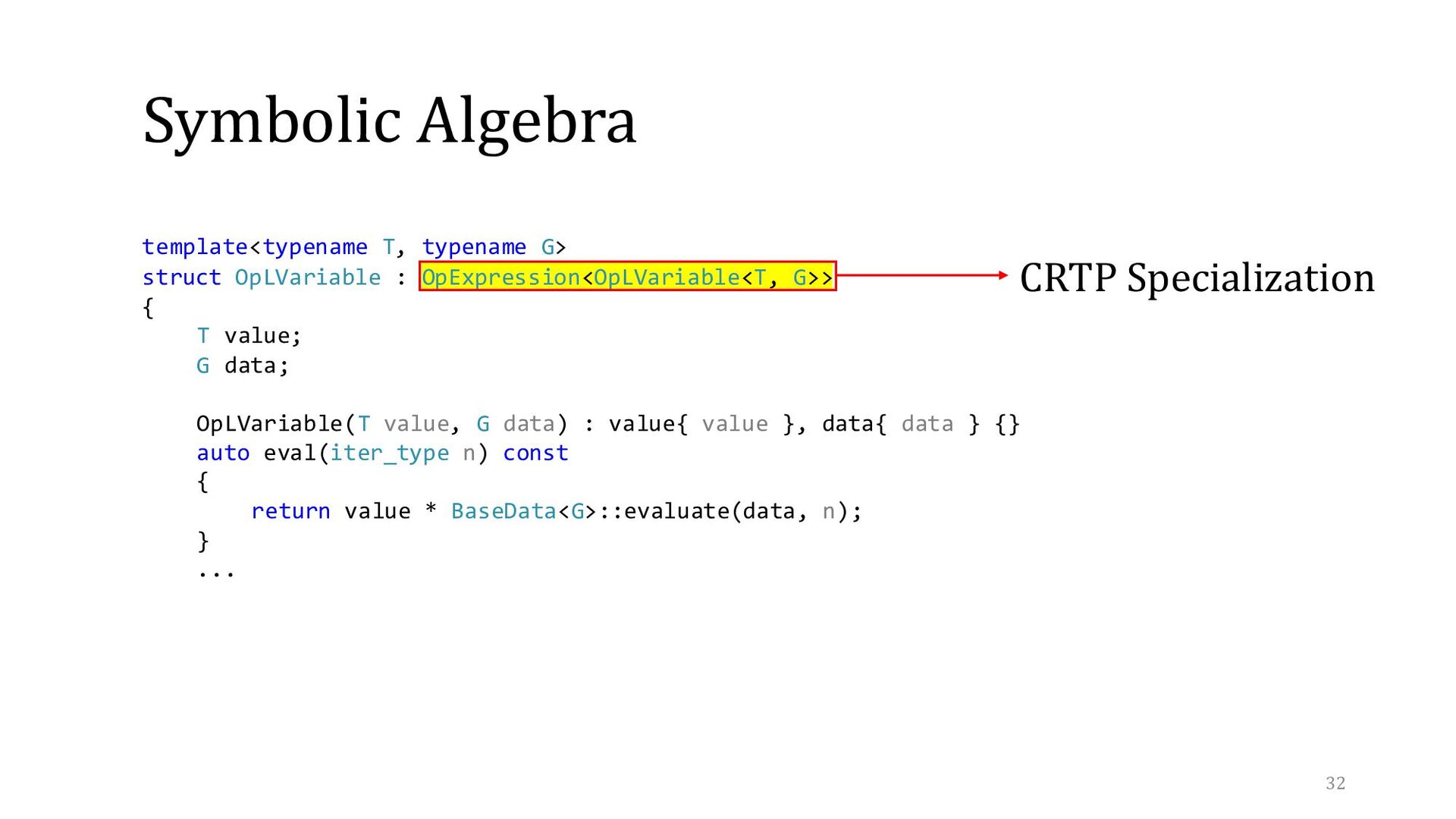
32. Symbolic Algebra CRTP Specialization template<typename T, typename G> struct OpLVariable : OpExpression<OpLVariable<T, G>> { T value; G data; OpLVariable(T value, G data) : value{ value }, data{ data } {} auto eval(iter_type n) const { return value * BaseData<G>::evaluate(data, n); } ... 32
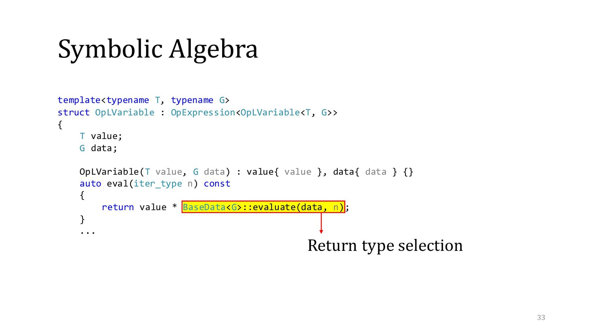
33. Symbolic Algebra Return type selection template<typename T, typename G> struct OpLVariable : OpExpression<OpLVariable<T, G>> { T value; G data; OpLVariable(T value, G data) : value{ value }, data{ data } {} auto eval(iter_type n) const { return value * BaseData<G>::evaluate(data, n); } ... 33
34. Symbolic Algebra • The CRTP is used with template argument deduction template<typename E1, typename E2> auto add(OpExpression<E1> const& a, OpExpression<E2> const& b) { ... } Template argument deduction 34
35. Symbolic Algebra • Library defines: → Distribution of multiplied terms → Collection of like terms → Multiplication by 0 or 1 → Addition/Subtraction by 0 → … 35
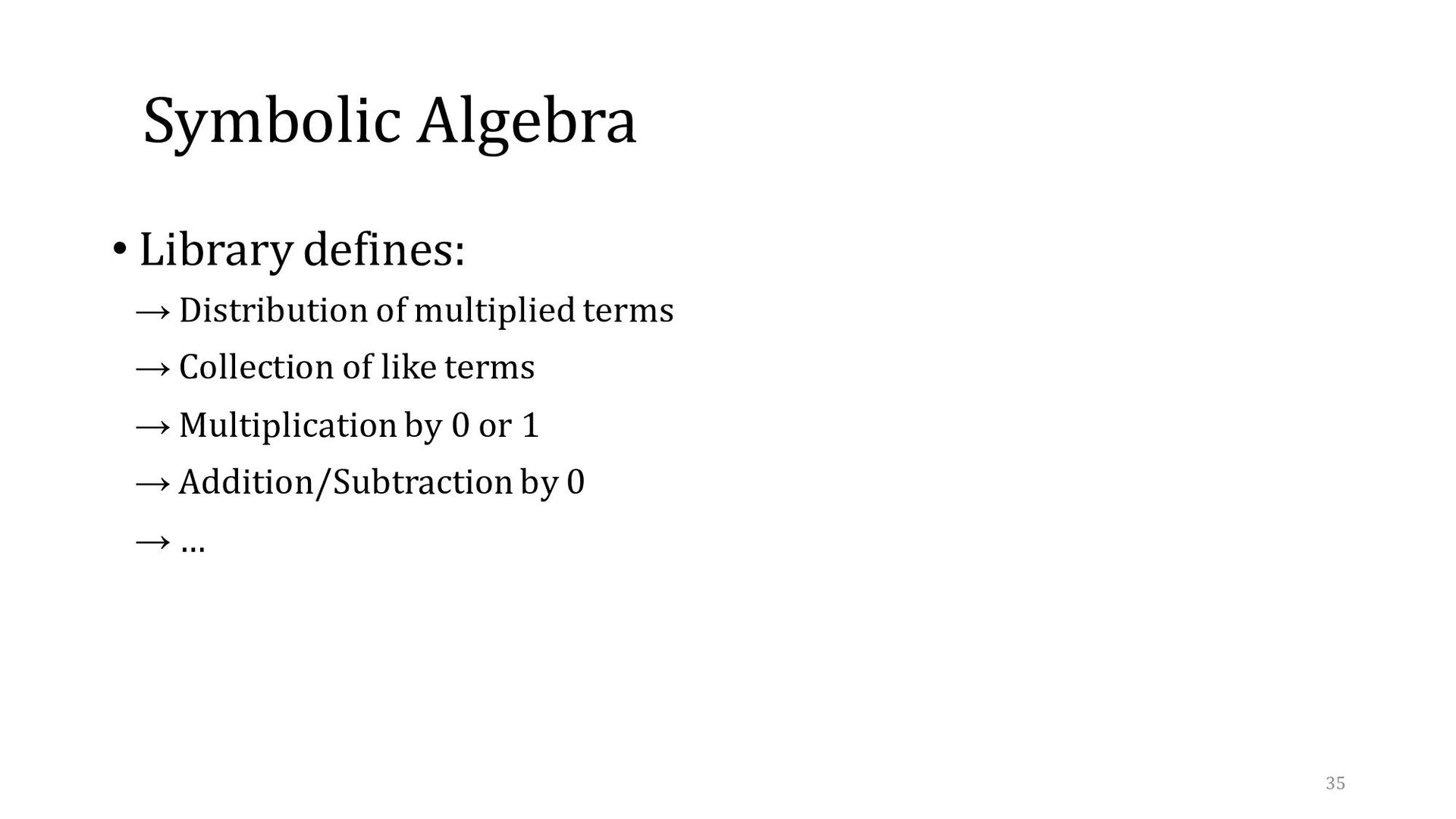
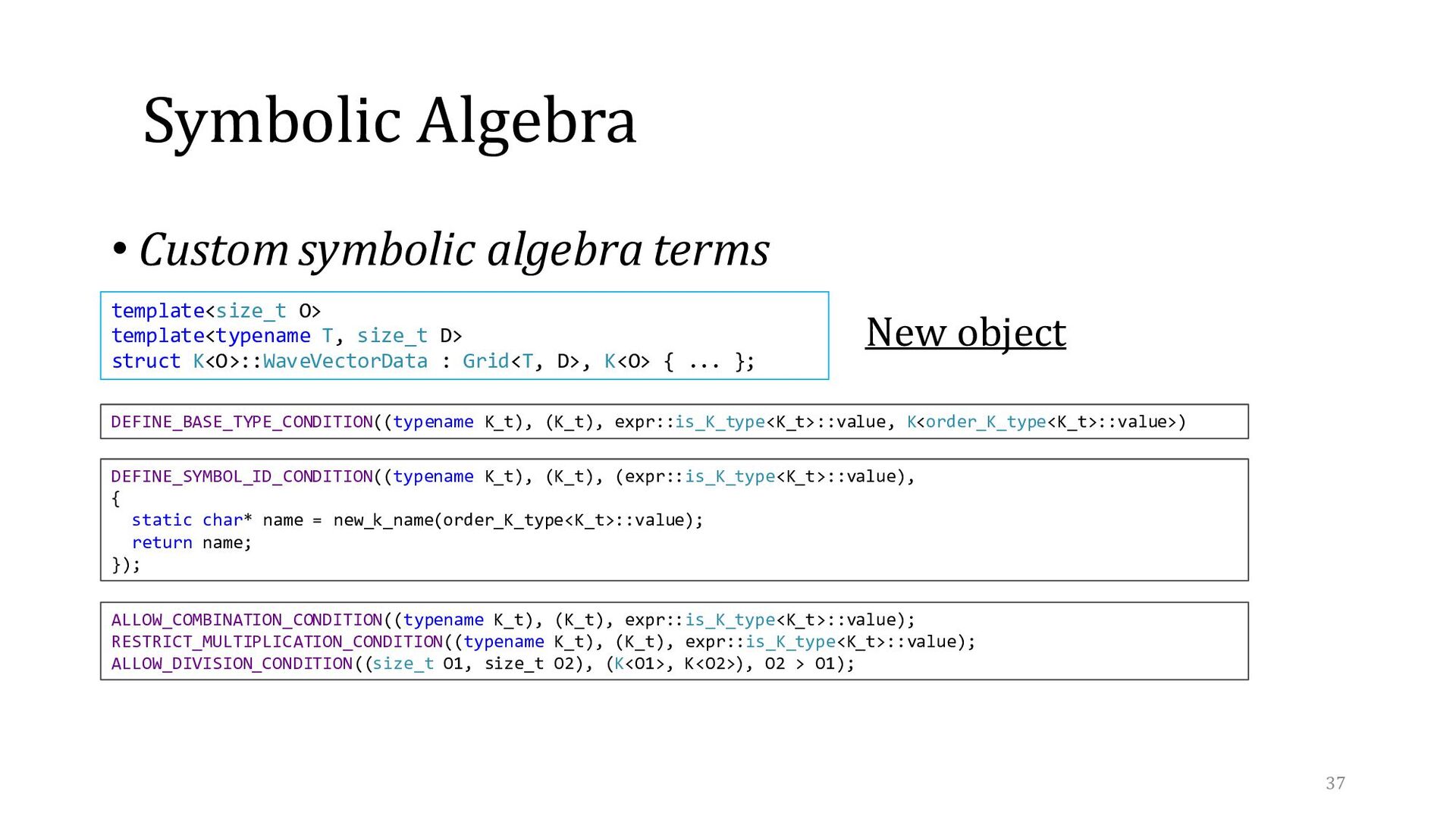
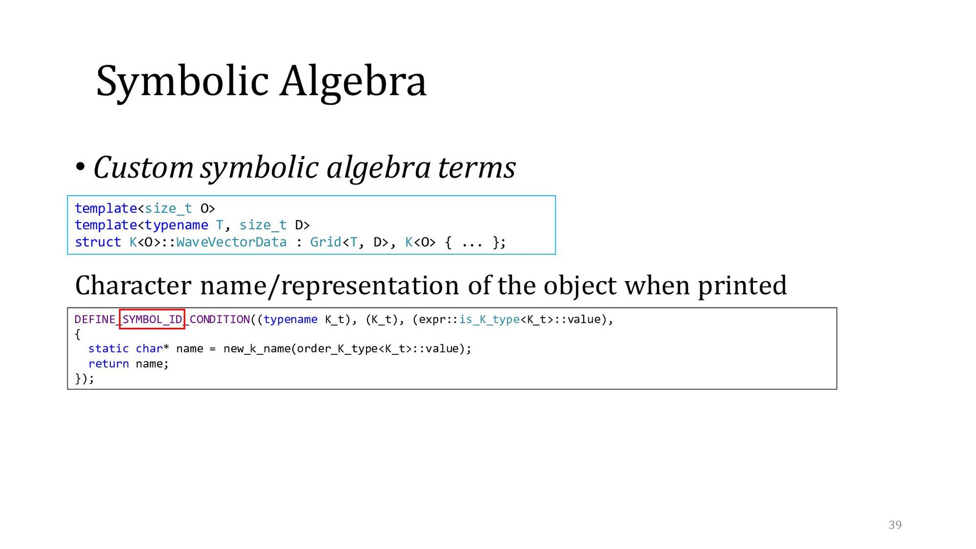
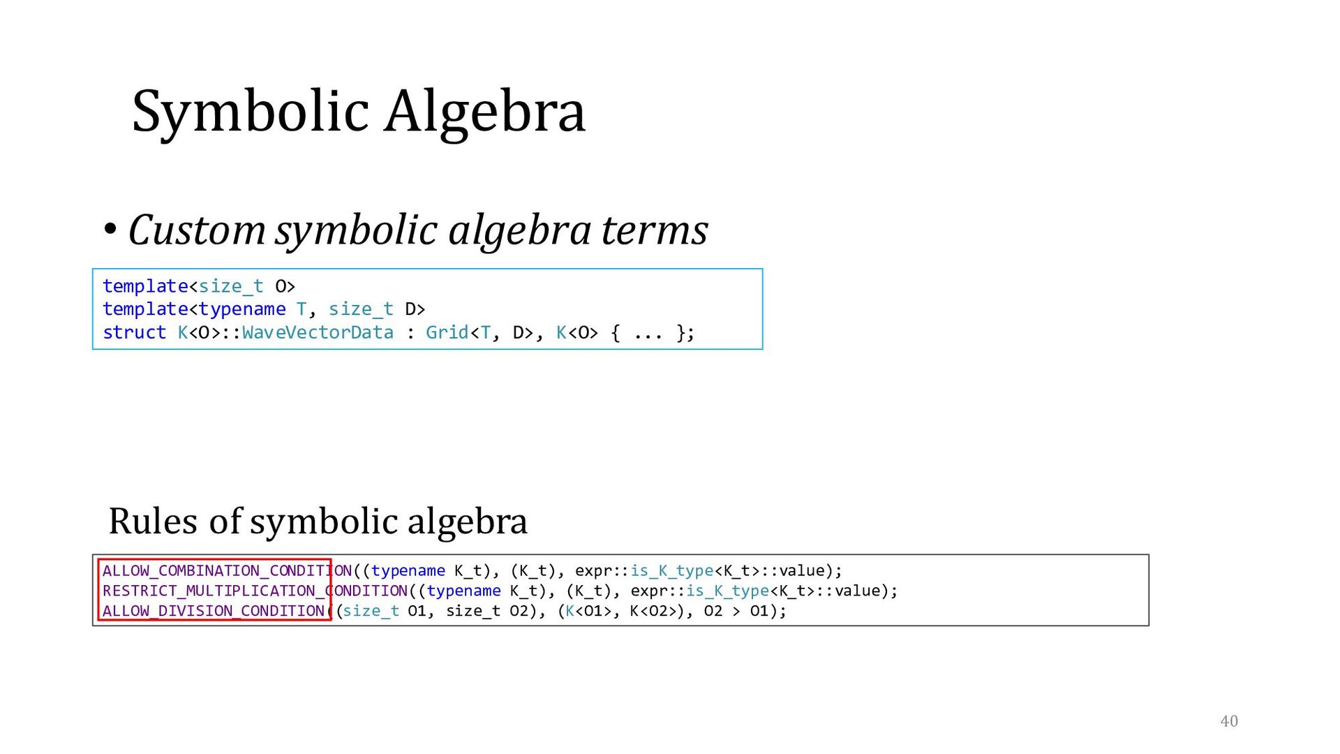
36. Symbolic Algebra • Library defines: → … → Defining a function with arguments → Factoring to cancel terms in a division → Transmuting terms → “Pretty printing” of expressions → Custom symbolic algebra terms 36
37. Symbolic Algebra • Custom symbolic algebra terms 37 DEFINE_BASE_TYPE_CONDITION((typename K_t), (K_t), expr::is_K_type<K_t>::value, K<order_K_type<K_t>::value>) DEFINE_SYMBOL_ID_CONDITION((typename K_t), (K_t), (expr::is_K_type<K_t>::value), { static char* name = new_k_name(order_K_type<K_t>::value); return name; }); ALLOW_COMBINATION_CONDITION((typename K_t), (K_t), expr::is_K_type<K_t>::value); RESTRICT_MULTIPLICATION_CONDITION((typename K_t), (K_t), expr::is_K_type<K_t>::value); ALLOW_DIVISION_CONDITION((size_t O1, size_t O2), (K<O1>, K<O2>), O2 > O1); template<size_t O> template<typename T, size_t D> struct K<O>::WaveVectorData : Grid<T, D>, K<O> { ... }; New object
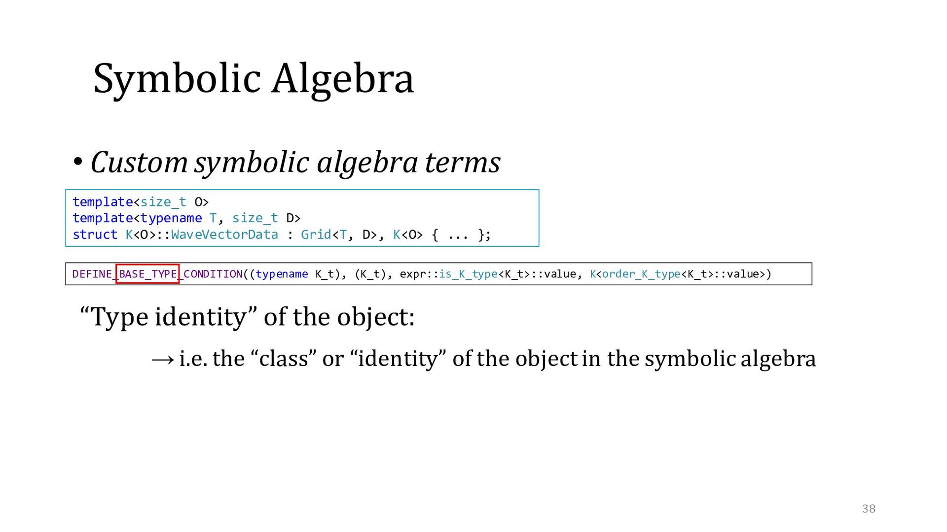
38. Symbolic Algebra • Custom symbolic algebra terms 38 DEFINE_BASE_TYPE_CONDITION((typename K_t), (K_t), expr::is_K_type<K_t>::value, K<order_K_type<K_t>::value>) template<size_t O> template<typename T, size_t D> struct K<O>::WaveVectorData : Grid<T, D>, K<O> { ... }; “Type identity” of the object: → i.e. the “class” or “identity” of the object in the symbolic algebra
39. Symbolic Algebra • Custom symbolic algebra terms 39 DEFINE_SYMBOL_ID_CONDITION((typename K_t), (K_t), (expr::is_K_type<K_t>::value), { static char* name = new_k_name(order_K_type<K_t>::value); return name; }); template<size_t O> template<typename T, size_t D> struct K<O>::WaveVectorData : Grid<T, D>, K<O> { ... }; Character name/representation of the object when printed
40. Symbolic Algebra • Custom symbolic algebra terms 40 ALLOW_COMBINATION_CONDITION((typename K_t), (K_t), expr::is_K_type<K_t>::value); RESTRICT_MULTIPLICATION_CONDITION((typename K_t), (K_t), expr::is_K_type<K_t>::value); ALLOW_DIVISION_CONDITION((size_t O1, size_t O2), (K<O1>, K<O2>), O2 > O1); template<size_t O> template<typename T, size_t D> struct K<O>::WaveVectorData : Grid<T, D>, K<O> { ... }; Rules of symbolic algebra
41. 4 | Simulation Examples 41
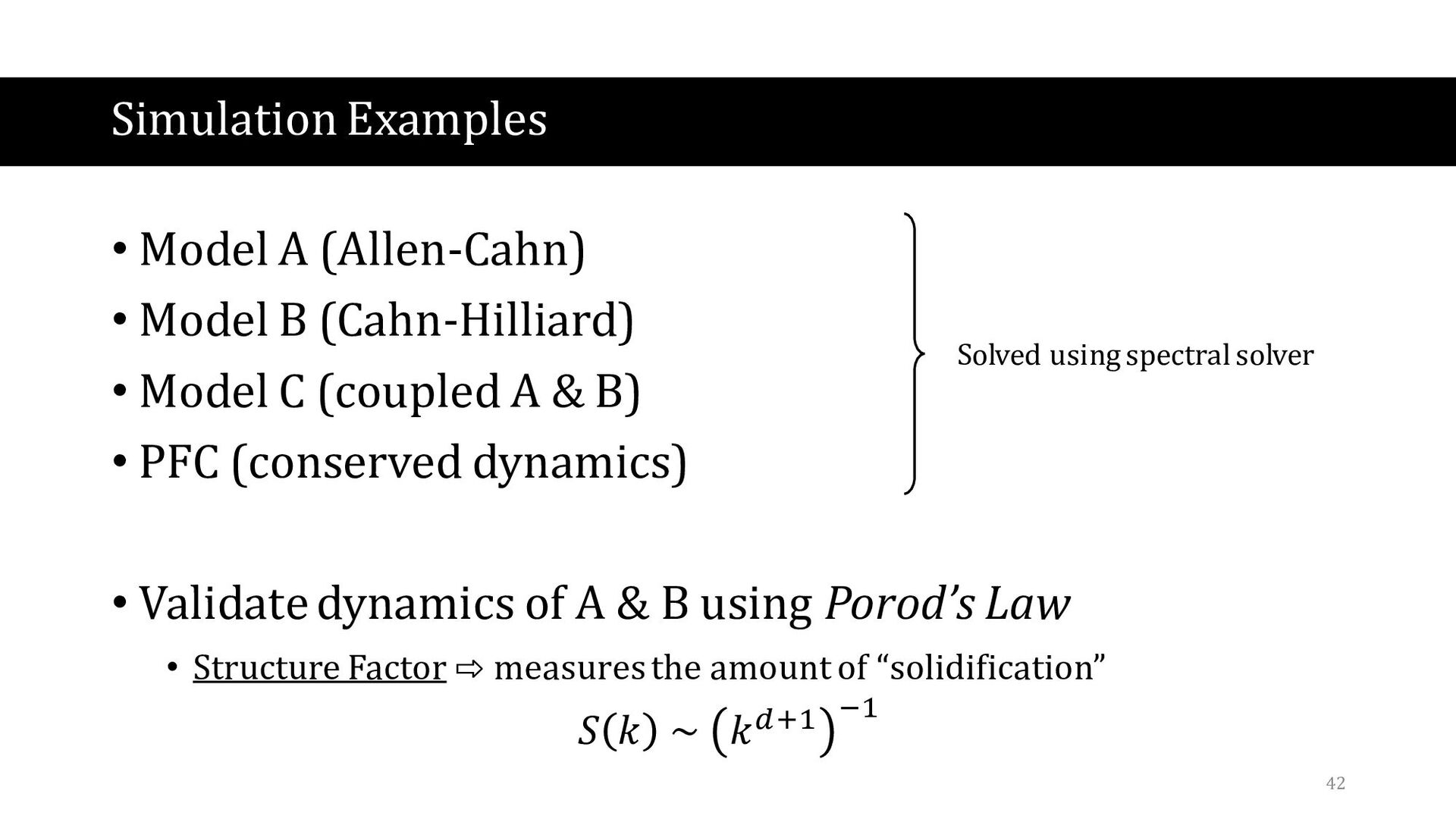
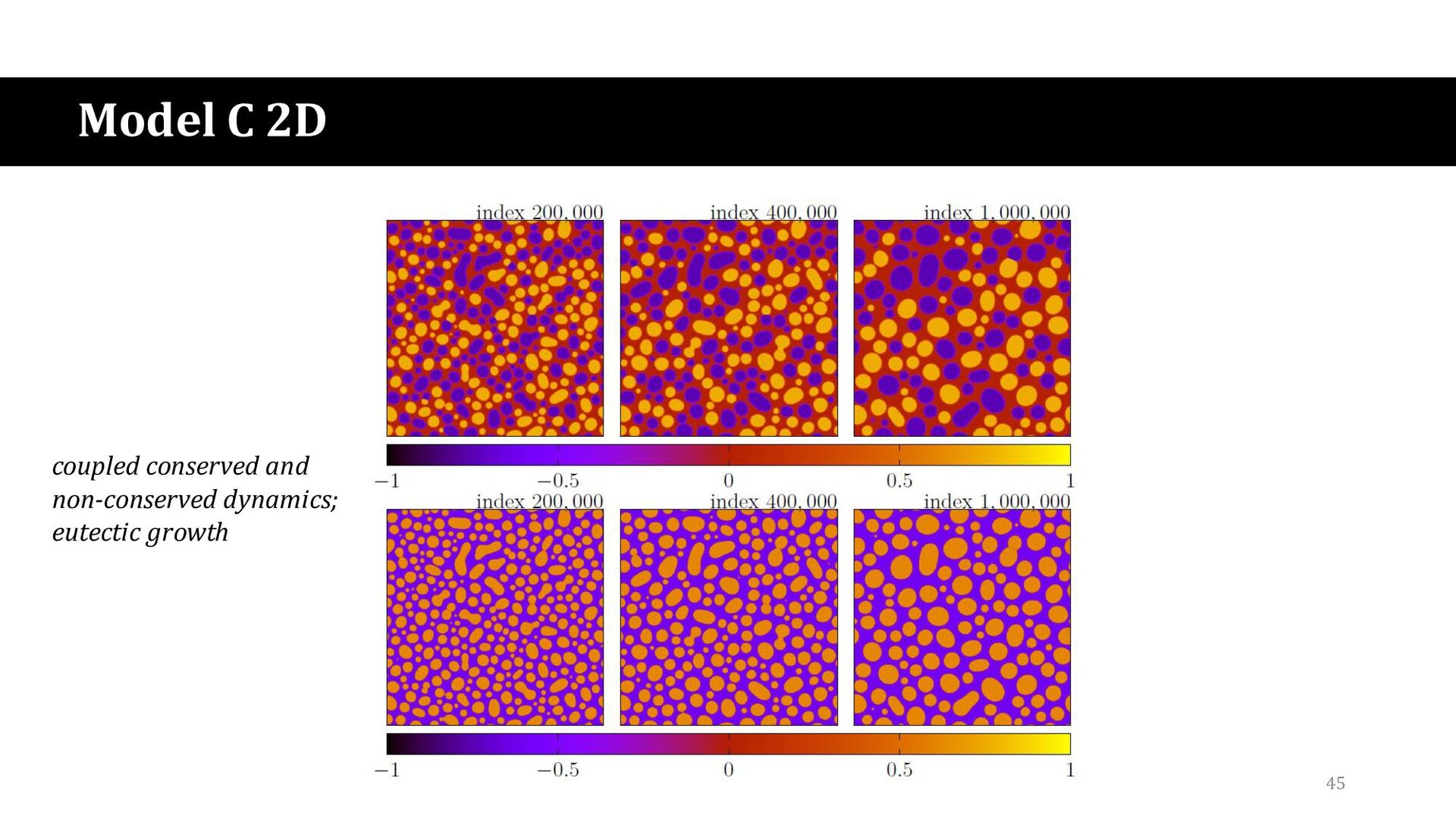
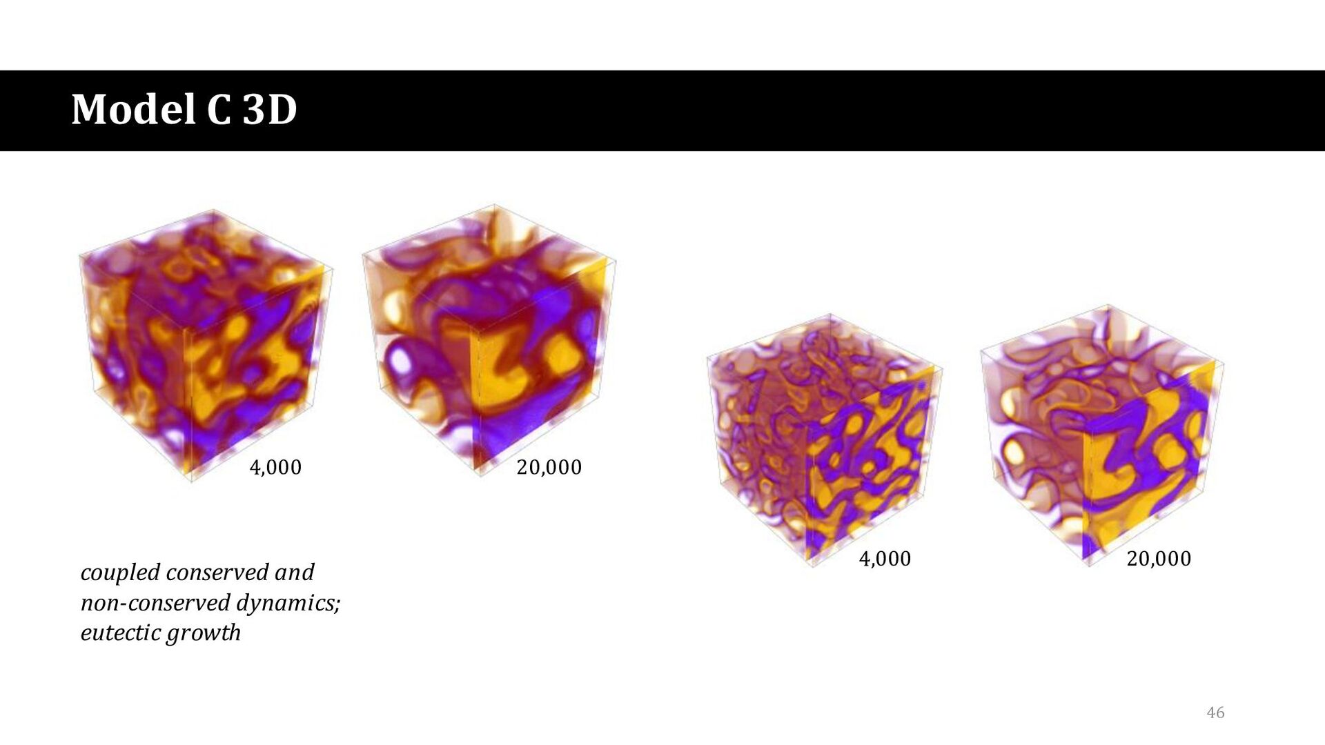
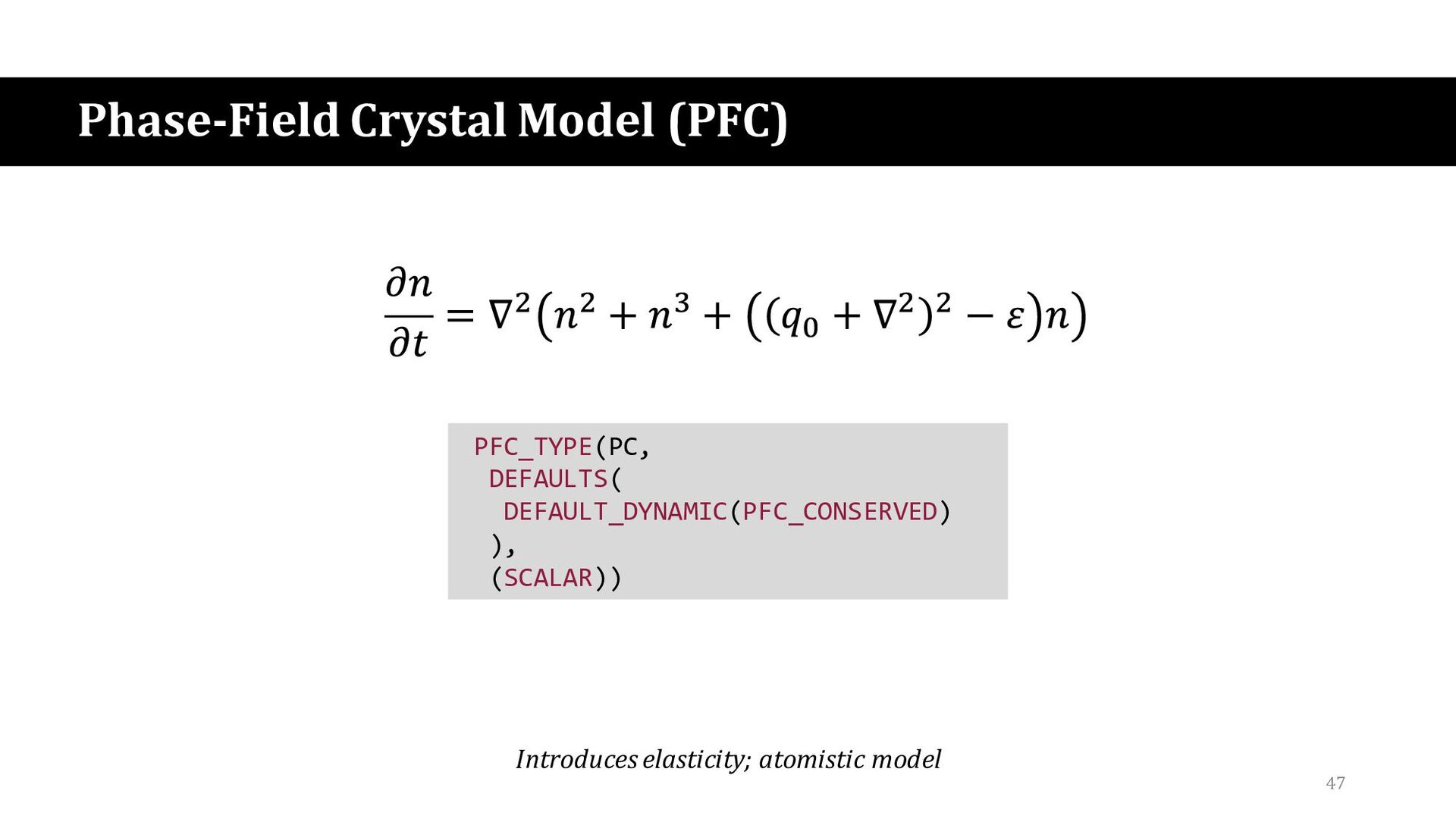
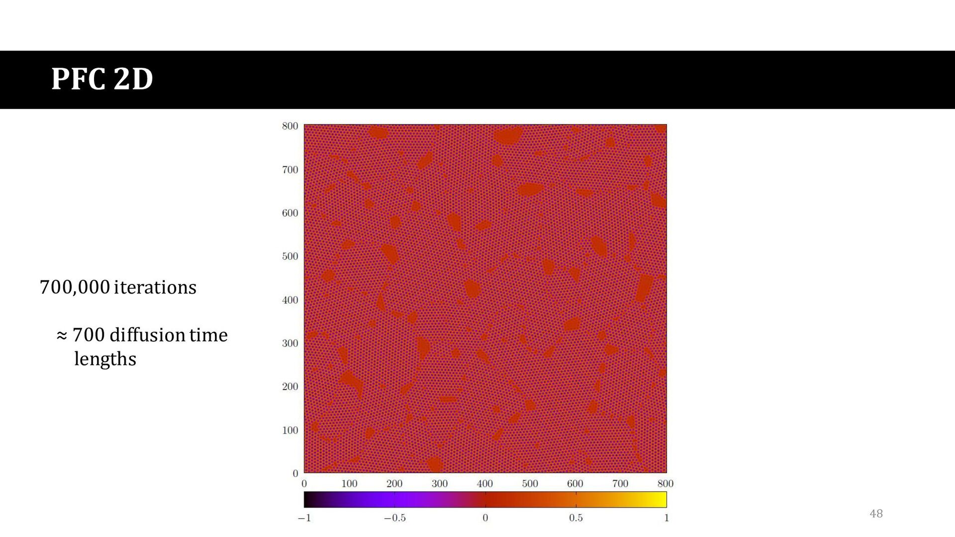
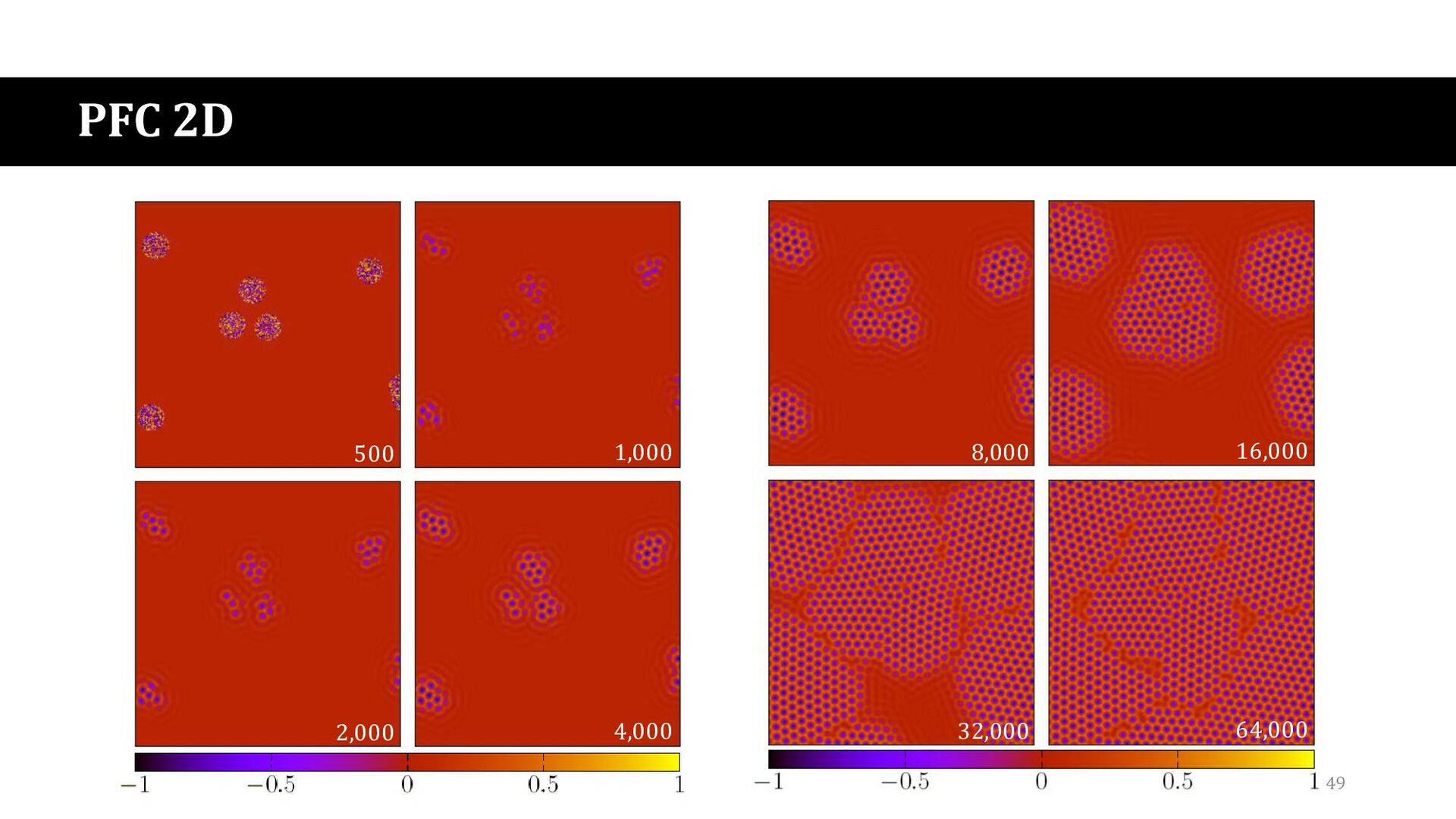
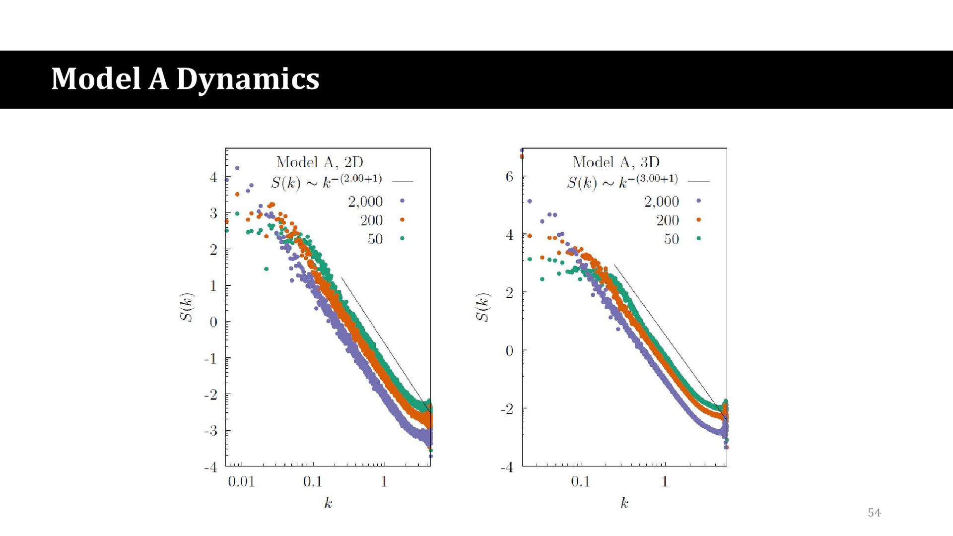
42. Simulation Examples • Model A (Allen-Cahn) • Model B (Cahn-Hilliard) • Model C (coupled A & B) • PFC (conserved dynamics) • Validate dynamics of A & B using Porod’s Law • Structure Factor ⇨ measures the amount of “solidification” 𝑆 𝑘 ~ 𝑘𝑑+1 −1 Solved using spectral solver 42
43. Simulation Examples • Runtime tests show: • Good scaling between 2D & 3D 43 S. A. Silber and M. Karttunen, “SymPhas —General Purpose Software for Phase-Field, Phase-Field Crystal, and Reaction-Diffusion Simulations,” Adv. Theory Simul., vol. 5, Art. no. 1, Dec. 2021.
44. Model C MODEL(MC, (SCALAR, SCALAR), MODEL_PREAMBLE_DEF( ( auto psi3 = c2 * psi * psi * psi, auto m3 = c4 * m * m * m) ), dpsi = lap(psi) + c1 * psi - psi3 + lit(2.) * c5 * psi * m, dm = -bilap(m) - lap(c3 * m - m3 + c5 * psi * psi))) coupled conserved and non-conserved dynamics; eutectic growth 44
45. Model C 2D coupled conserved and non-conserved dynamics; eutectic growth 45
46. Model C 3D coupled conserved and non-conserved dynamics; eutectic growth 4,000 20,000 4,000 20,000 46
47. Phase-Field Crystal Model (PFC) PFC_TYPE(PC, DEFAULTS( DEFAULT_DYNAMIC(PFC_CONSERVED) ), (SCALAR)) Introduces elasticity; atomistic model 47
48. PFC 2D 700,000 iterations ≈ 700 diffusion time lengths 48
49. PFC 2D 500 1,000 2,000 4,000 8,000 16,000 32,000 64,000 49
50. PFC 3D 70,000 iterations 50
51. Model A non-conserved dynamics; chemical potential driven phase transition MODEL(MA, (SCALAR), MODEL_DEF( dpsi = lap(psi) + (c1 - c2 * psi * psi) * psi)) 51
52. Model A 2D non-conserved dynamics; chemical potential driven phase transition 52
53. Model A 3D non-conserved dynamics; chemical potential driven phase transition 400 2000 800 53
54. Model A Dynamics 54
55. Model B MODEL(MB, (SCALAR), MODEL_DEF( dm = -bilap(m) - lap(c1 - c2 * m * m) * m)) conserved dynamics; chemical potential driven phase transition 55
56. Model B 2D conserved dynamics; chemical potential driven phase transition 56
57. Model B 3D conserved dynamics; chemical potential driven phase transition 4,000 20,000 8,000 57
58. Model B Dynamics 58
59. Acknowledgements • Western University • NSERC CGSM Scholarship • Mitacs GlobalLink Travel Grant • Aalto University 59
60. Appendix Slides 60
61. • Expression trees fulfill these needs … a construct that is both evaluable & modifiable Symbolic Algebra 1 2 + + ÷ 6 𝜓 8 × + 4 61
62. SymPhas API & Implementation • A SymPhas implementation in 22 lines: #include "symphas.h" MODEL(EX, (SCALAR), MODEL_DEF(dop(1) = lap(op(1)) + (c1 - lit (4.) * c2 * op(1) * op(1)) * op(1))) int main(int argc , char* argv []) { double dt = 0.1; symphas::problem_parameters_type pp{ 1 }; symphas::b_data_type bdata; symphas::init_data_type tdata{ Inside::UNIFORM, { -1, 1 } }; symphas::interval_data_type vdata; symphas::interval_element_type interval; interval.set_interval_count(0, 128, 128); bdata[Side::LEFT] = BoundaryType::PERIODIC; bdata[Side::RIGHT] = BoundaryType::PERIODIC; bdata[Side::TOP] = BoundaryType::PERIODIC; bdata[Side::BOTTOM] = BoundaryType::PERIODIC; vdata[Axis::X] = interval; vdata[Axis::Y] = interval; pp.set_boundary_data(&bdata); pp.set_initial_data(&tdata); pp.set_interval_data(&vdata); pp.set_problem_time_step(dt); model_EX_t<2, SolverSP<Stencil2d2h<5, 9, 6>>> model{ pp }; symphas::find_solution(model, dt, 50);} Define new Model . ⊳ Solve phase-field model ⊳ Boundary conditions ⊳ Initial conditions … ⊳ System size … . ⊳ Initialize problem … ⊳ 62
63. Problem Representation Uniform Grid Uniform Grid Uniform Grid 63
64. Problem Representation System Uniform Grid System Uniform Grid System Uniform Grid 64 *Changes based on use of io module
65. 4 | Numerical Solvers 65
66. Numerical Solvers • Phase-field data, 𝜓, represented by a regular grid → Cartesian coordinate system,Δ𝑥 (× Δ𝑦 (× Δ𝑧)) → Each element represents the average of the phase-field Numerical solution in 1D denoted: 𝜓𝑗 𝑛 ≔ 𝜓 𝑥 = 𝑗Δ𝑥,𝑡 = 𝑛Δ𝑡 • SymPhas implements two numerical solvers: → Forward-Time Central-Space (FTCS) (Forward Euler) Solver → Semi-implicit Fourier spectral solver Δ𝑦 Δ𝑥 Δz 𝑥 𝑦 𝑧 66
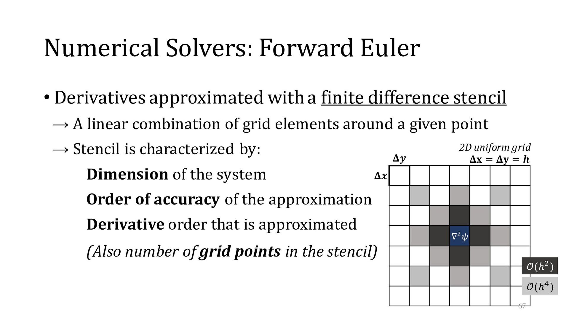
67. Numerical Solvers: Forward Euler • Derivatives approximated with a finite difference stencil → A linear combination of grid elements around a given point → Stencil is characterized by: Dimension of the system Order of accuracy of the approximation Derivative order that is approximated (Also number of grid points in the stencil) ∇2𝜓 2D uniform grid 𝒪(ℎ4) 𝒪(ℎ2) 𝚫𝒙 𝚫𝒚 𝚫𝐱 = 𝚫𝐲 = 𝒉 67
68. Numerical Solvers: Forward Euler & periodic BC • Approximation of 𝝏 𝝏𝒕 𝝍 ≈ 𝜓𝑗 𝑛+1 − 𝜓𝑗 𝑛 Δ𝑡 • Approximation of 𝛁𝟐𝝍 ≈ 𝜓𝑗+1 𝑛 − 2𝜓𝑗 𝑛 + 𝜓𝑗−1 𝑛 ℎ2 Resulting Scheme: ∇2𝜓 1D grid 𝒉 ⊲ 𝒪 Δ𝑡 accurate ⊲ 𝒪 ℎ2 accurate 68
69. Numerical Solvers: Forward Euler • Derivatives approximated with a finite difference stencil → A stencil: template object can be readily extended specializations interchangeable with generalizations The whole point: template<size_t DD, size_t OA> struct SelfSelectingStencil 69 len_type dims[]{ 10, 10 }; auto stencil = SelfSelectingStencil<2, 2>::Points<9, 13, 6>{dims, 1.0};
70. Numerical Solvers: Forward Euler • Derivatives approximated with a finite difference stencil → A stencil combines an interface and general implementation 70 template<typename Sp> struct Stencil { template <typename T> auto laplacian(T * const v) const { return (*static_cast<const Sp*>(this)).laplacian(v); } template <typename T> auto bilaplacian(T * const v) const ... template <typename T> auto gradlaplacian(T * const v) const ... template<typename T> auto gradient(T * const v) const }; template<size_t DD, size_t OA = DEFAULT_STENCIL_ACCURACY> struct GeneralizedStencil { len_type dims[DD]; double divh; GeneralizedStencil(const len_type* dims, double h) : divh{ 1. / h } { std::copy(dims, dims + DD, this->dims); } template<size_t OD, typename T> auto apply(T* const v) const { return *v; } }; +
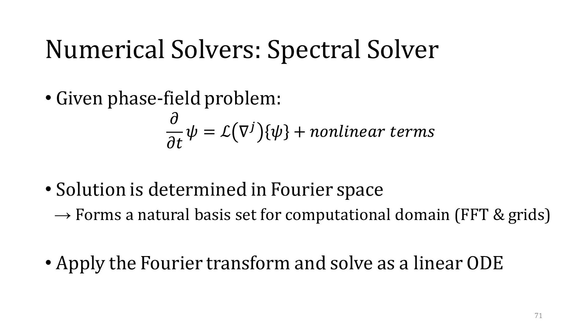
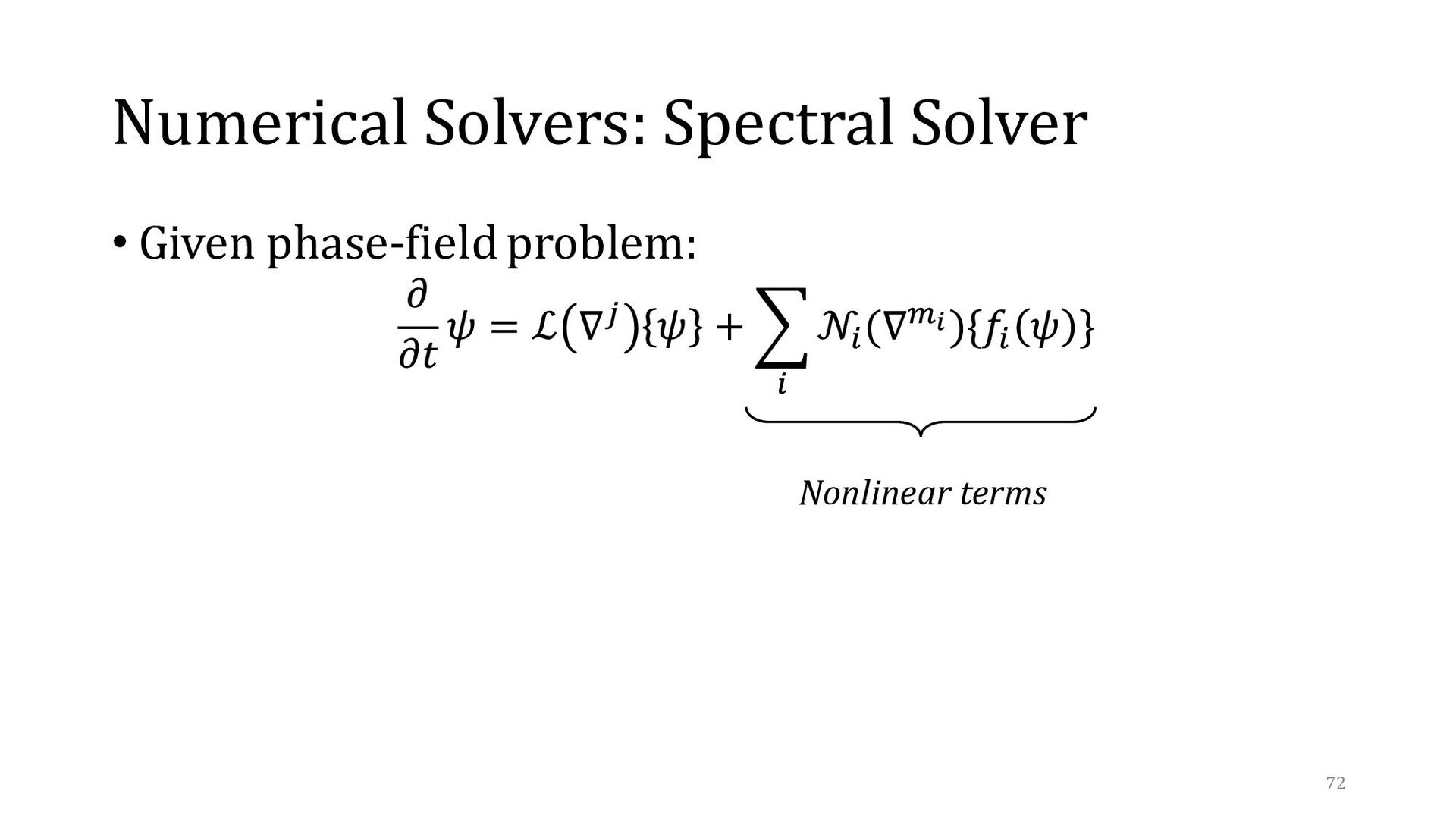
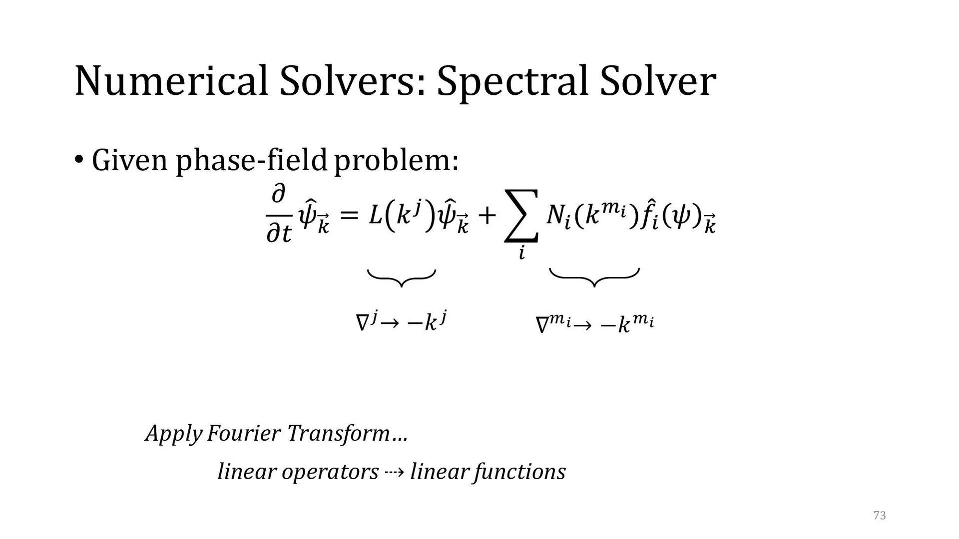
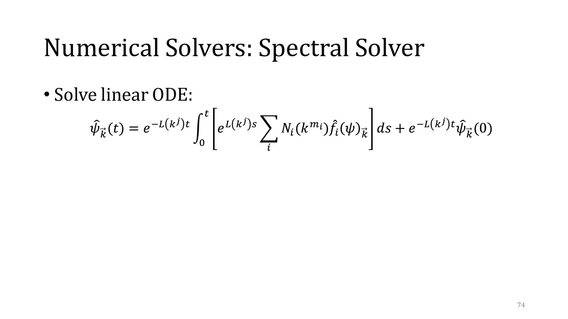
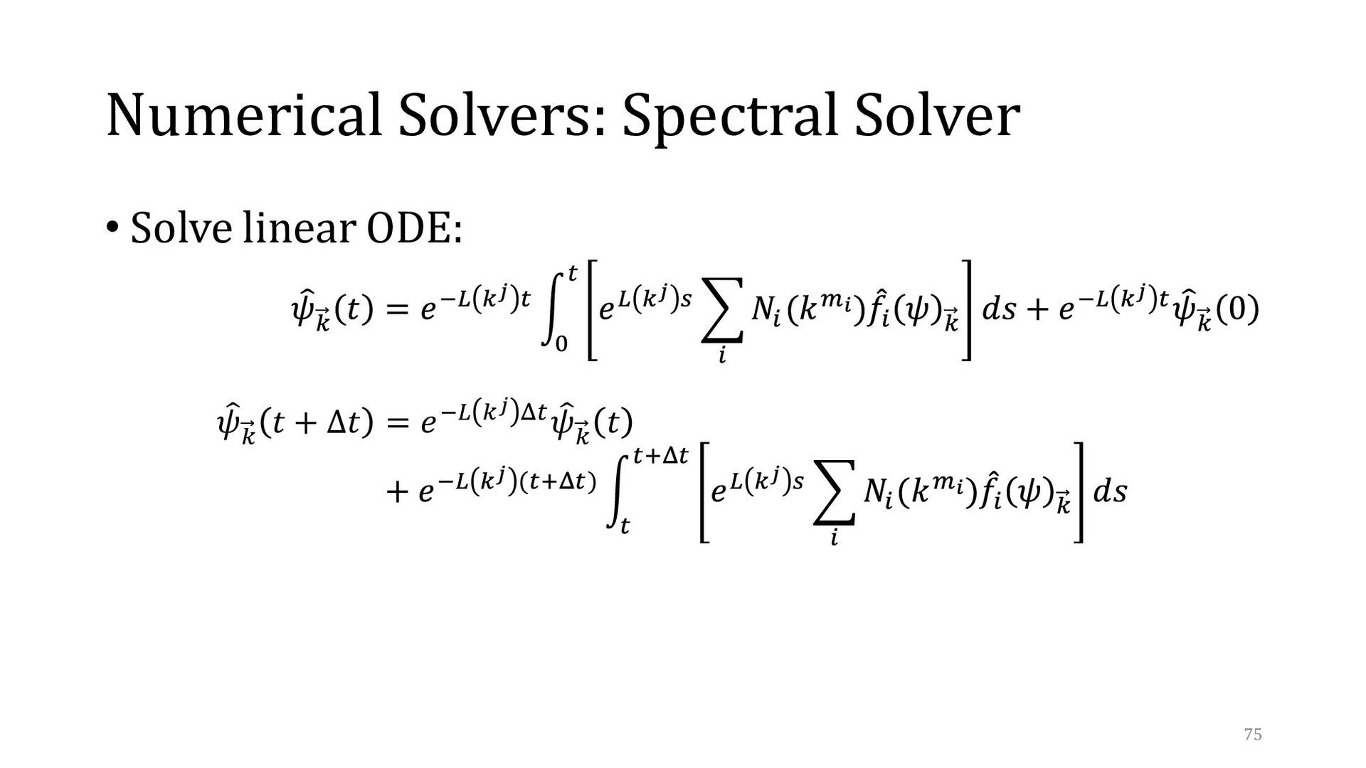
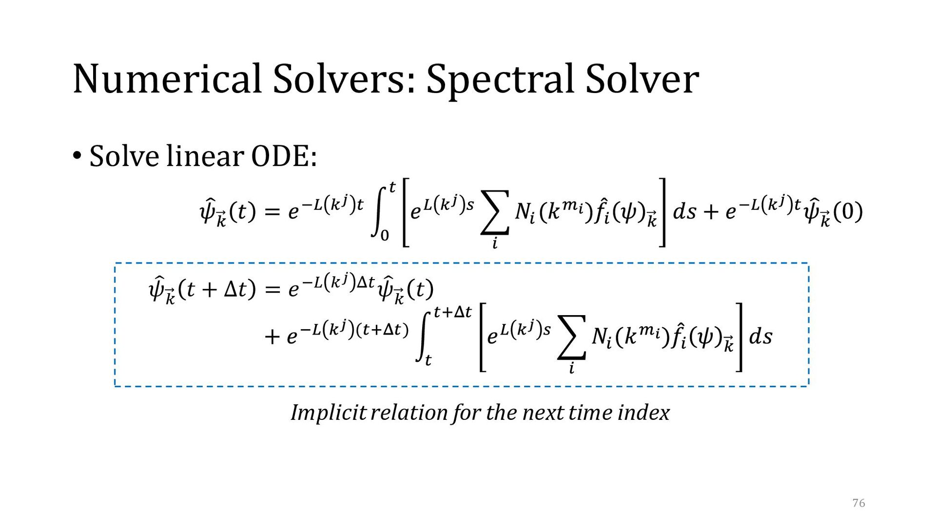
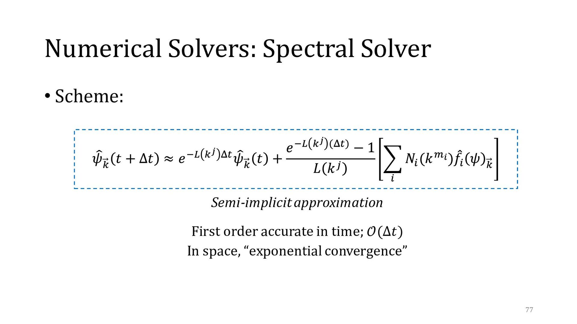
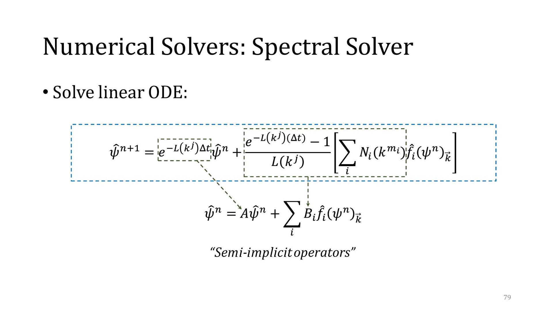
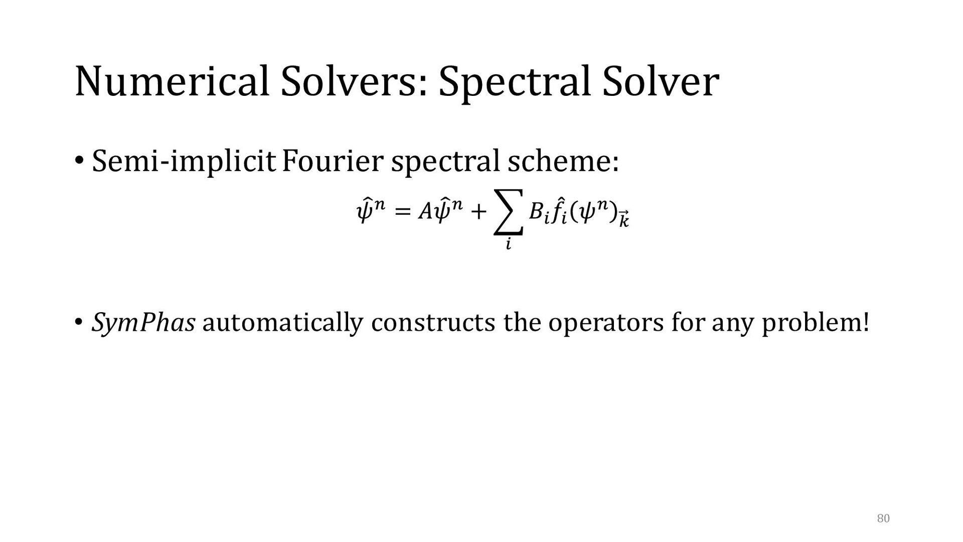
71. Numerical Solvers: Spectral Solver • Given phase-field problem: • Solution is determined in Fourier space → Forms a natural basis set for computational domain (FFT & grids) • Apply the Fourier transform and solve as a linear ODE 71
72. Numerical Solvers: Spectral Solver • Given phase-field problem: Nonlinear terms 72
73. Numerical Solvers: Spectral Solver • Given phase-field problem: Apply Fourier Transform… linear operators ⇢ linear functions ∇𝑗→ −𝑘𝑗 ∇𝑚𝑖→ −𝑘𝑚𝑖 73
74. Numerical Solvers: Spectral Solver • Solve linear ODE: 74
75. Numerical Solvers: Spectral Solver • Solve linear ODE: ෠ 𝜓 𝑘 𝑡 + Δ𝑡 = 𝑒−𝐿 𝑘𝑗 Δ𝑡 ෠ 𝜓 𝑘 𝑡 75
76. Numerical Solvers: Spectral Solver • Solve linear ODE: ෠ 𝜓 𝑘 𝑡 + Δ𝑡 = 𝑒−𝐿 𝑘𝑗 Δ𝑡 ෠ 𝜓 𝑘 𝑡 Implicit relation for the next time index 76
77. Numerical Solvers: Spectral Solver • Scheme: Semi-implicit approximation First order accurate in time; 𝒪(Δ𝑡) In space, “exponential convergence” 77
78. Numerical Solvers: Spectral Solver • Determine scheme: Semi-implicit spectral Fourier scheme First order accurate in time; 𝒪(Δ𝑡) In space, “exponential convergence” 78
79. Numerical Solvers: Spectral Solver • Solve linear ODE: “Semi-implicit operators” 79
80. Numerical Solvers: Spectral Solver • Semi-implicit Fourier spectral scheme: • SymPhas automatically constructs the operators for any problem! 80