Fitting Free Energies with Neural Networks

Transcript

1. Fitting Free Energies with Neural Networks Daniel Schwen Idaho National Laboratory
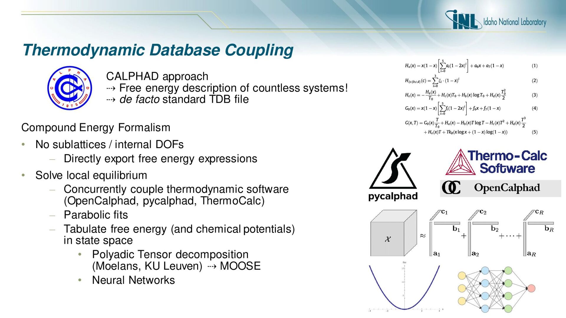
2. Thermodynamic Database Coupling CALPHAD approach ⇢ Free energy description of countless systems! ⇢ de facto standard TDB file Compound Energy Formalism • No sublattices / internal DOFs – Directly export free energy expressions • Solve local equilibrium – Concurrently couple thermodynamic software (OpenCalphad, pycalphad, ThermoCalc) – Parabolic fits – Tabulate free energy (and chemical potentials) in state space • Polyadic Tensor decomposition (Moelans, KU Leuven) ⇢ MOOSE • Neural Networks
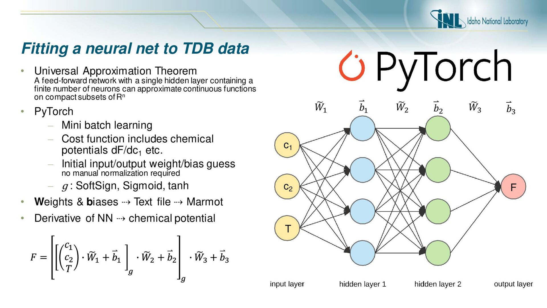
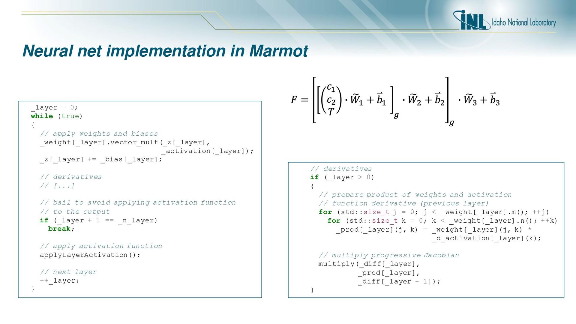
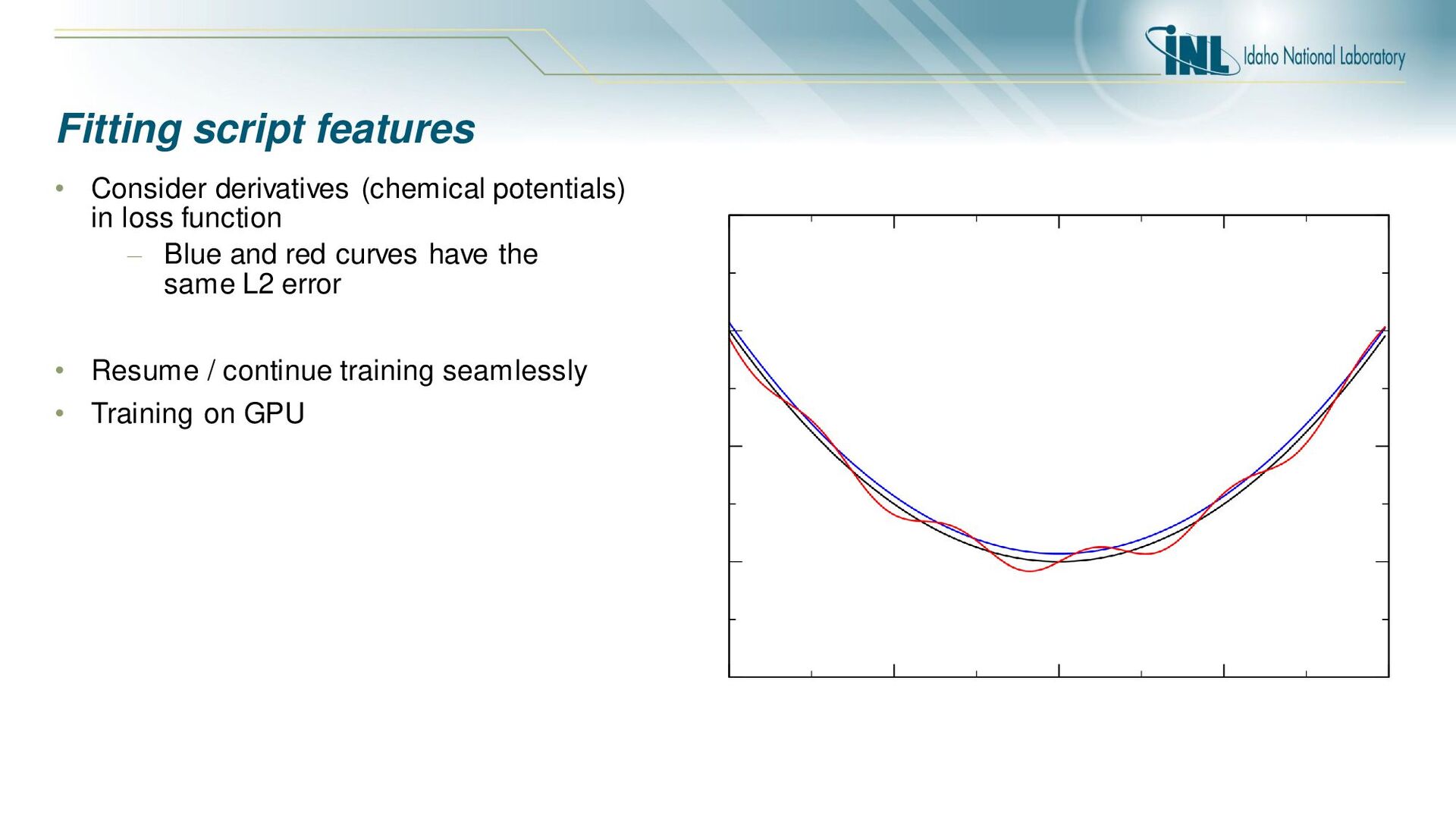
3. Fitting a neural net to TDB data c1 c2 T F • Universal Approximation Theorem A feed-forward network with a single hidden layer containing a finite number of neurons can approximate continuous functions on compact subsets of Rn • PyTorch – Mini batch learning – Cost function includes chemical potentials dF/dc1 etc. – Initial input/output weight/bias guess no manual normalization required – ɡ : SoftSign, Sigmoid, tanh • Weights & biases ⇢ Text file ⇢ Marmot • Derivative of NN ⇢ chemical potential ෩ 𝑊1 ෩ 𝑊2 ෩ 𝑊3 𝑏1 𝑏2 𝑏3
4. Neural net implementation in Marmot _layer = 0; while (true) { // apply weights and biases _weight[_layer].vector_mult(_z[_layer], _activation[_layer]); _z[_layer] += _bias[_layer]; // derivatives // [...] // bail to avoid applying activation function // to the output if (_layer + 1 == _n_layer) break; // apply activation function applyLayerActivation(); // next layer ++_layer; } // derivatives if (_layer > 0) { // prepare product of weights and activation // function derivative (previous layer) for (std::size_t j = 0; j < _weight[_layer].m(); ++j) for (std::size_t k = 0; k < _weight[_layer].n(); ++k) _prod[_layer](j, k) = _weight[_layer](j, k) * _d_activation[_layer](k); // multiply progressive Jacobian multiply(_diff[_layer], _prod[_layer], _diff[_layer - 1]); }
5. Fitting script (PyTorch) schwd$ ./fit_neural_net.py --help usage: fit_neural_net.py [-h] [-c] [-o OUTPUT_STATUS] [-O OUTPUT_MODEL] [-e EPOCHS] [-m MINI_BATCH] [-H HIDDEN_LAYER_NODES] [-n HIDDEN_LAYER_COUNT] [-r LEARNING_RATE] datafile inputs outputs Fit a neural network to a Gibbs free energy. positional arguments: datafile Text file with columns for the inputs, free energy, and (optionally) chemical potential data. inputs Number of input nodes outputs Number of input nodes optional arguments: -h, --help show this help message and exit -c, --use_chemical_potentials -o OUTPUT_STATUS, --output_status OUTPUT_STATUS Epoch interval for outputting the loss function value to screen and disk -O OUTPUT_MODEL, --output_model OUTPUT_MODEL Epoch interval for outputting the NN torch model to disk -e EPOCHS, --epochs EPOCHS Epochs to run for training (50000) -m MINI_BATCH, --mini_batch MINI_BATCH Mini batch size (128) -H HIDDEN_LAYER_NODES, --hidden_layer_nodes HIDDEN_LAYER_NODES Number of nodes per hidden layer (20) -n HIDDEN_LAYER_COUNT, --hidden_layer_count HIDDEN_LAYER_COUNT Number of hidden layers (2) -r LEARNING_RATE, --learning_rate LEARNING_RATE Learning rate meta parameter (1e-5) layers = [torch.nn.Linear(D_in, H), activation()] for i in range(1, hidden_layer_count): layers += [torch.nn.Linear(H, H), activation()] layers += [torch.nn.Linear(H, D_out)] model = torch.nn.Sequential(*layers) # random weight seeding model.apply(weights_init) # apply input/output data normalization # to weights and biases adjust_weights() optimizer = torch.optim.Adam(model.parameters(), lr=learning_rate) for epoch in range(n_epochs): # generate a new permutation of the training set permutation = torch.randperm(x.size()[0]) # iterate over mini batches for i in range(0,x.size()[0], batch_size): …
6. Fitting script features • Consider derivatives (chemical potentials) in loss function – Blue and red curves have the same L2 error • Resume / continue training seamlessly • Training on GPU
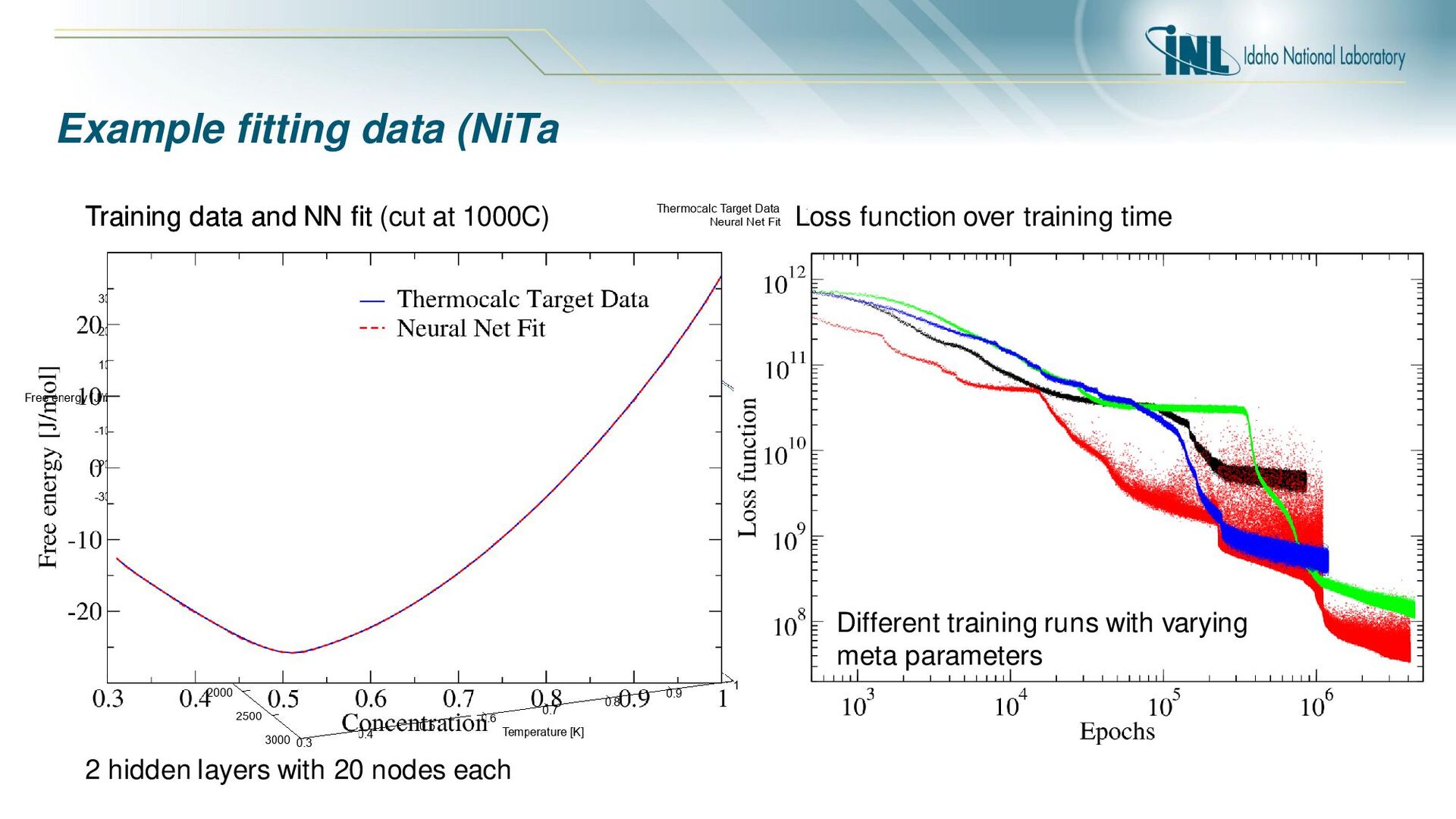
7. Example fitting data (NiTa Training data and NN fit (cut at 1000C) Loss function over training time 2 hidden layers with 20 nodes each Different training runs with varying meta parameters Training data and NN fit
8. Fitting data from a known function Loss function over training time 2 hidden layers with 20 nodes each 𝑓 = 𝑐 1 − 𝑐 + 10−3𝑇(𝑐 log𝑐 + 1 − 𝑐 log 1 − 𝑐 ) 400,000 epochs 1,500 minibatch size Learning rate 10-5 Trained on GPU (~1.5h)
9. Neural net free energy • Simple double well energy, 1 component + 1 temperature input node • Fit using 2 hidden layers with 20 neurons each Analytical Free Energy Neural Net Free Energy Difference
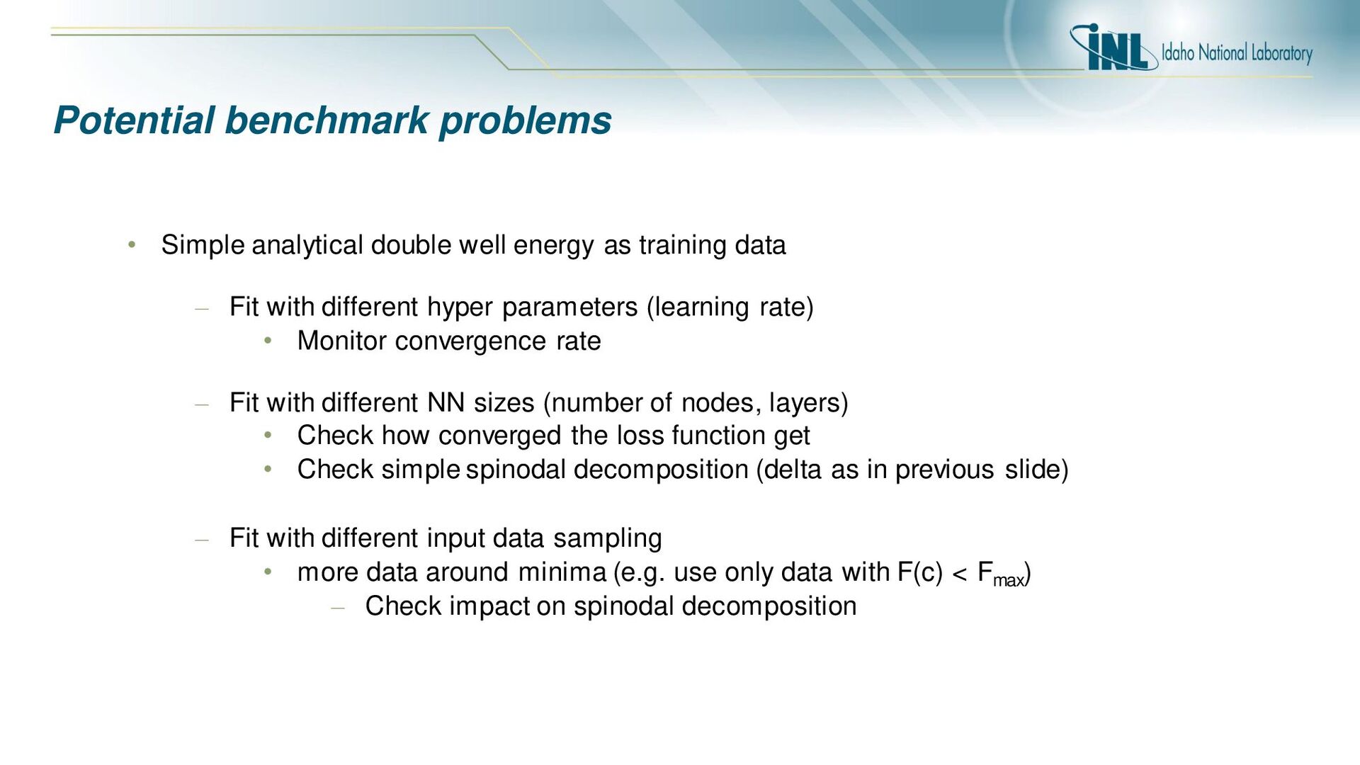
10. Potential benchmark problems • Simple analytical double well energy as training data – Fit with different hyper parameters (learning rate) • Monitor convergence rate – Fit with different NN sizes (number of nodes, layers) • Check how converged the loss function get • Check simple spinodal decomposition (delta as in previous slide) – Fit with different input data sampling • more data around minima (e.g. use only data with F(c) < Fmax ) – Check impact on spinodal decomposition