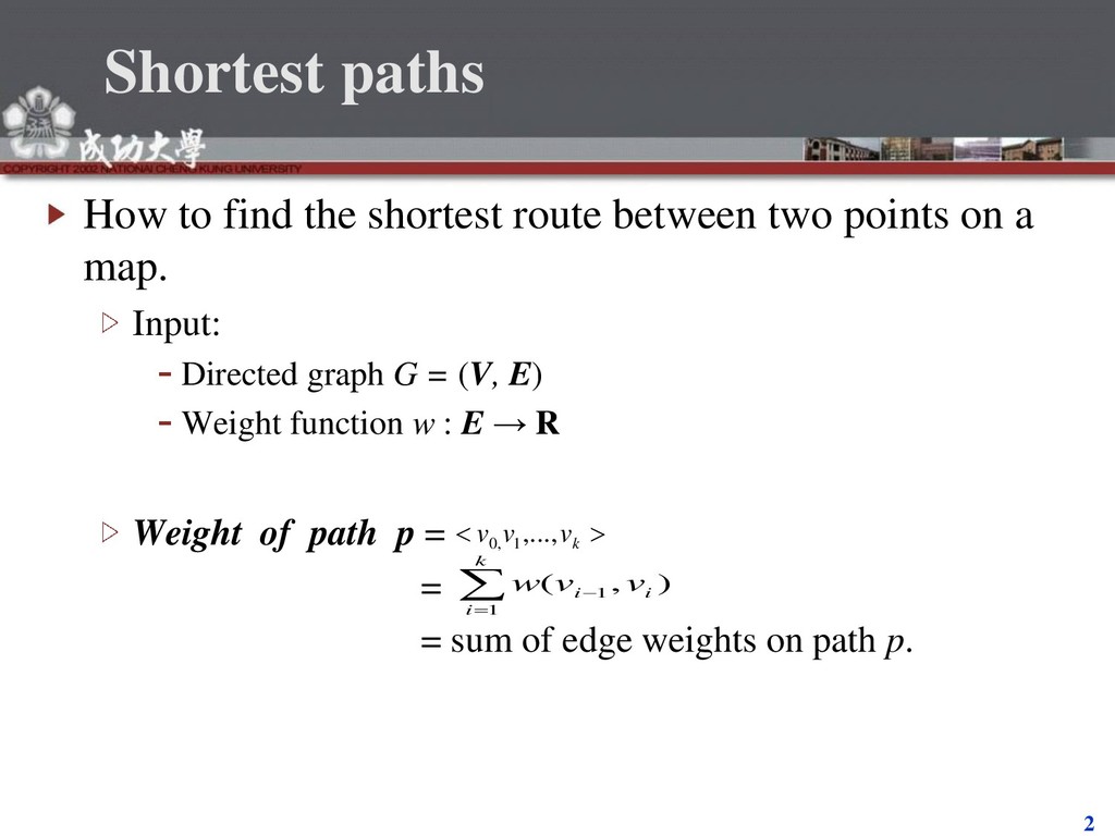
two points on a map. Input: Directed graph G = (V, E) Weight function w : E → R Weight of path p = = = sum of edge weights on path p. k v v v ,..., 1 , 0 k i i i v v w 1 1 ) , (
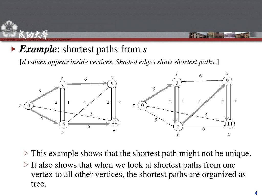
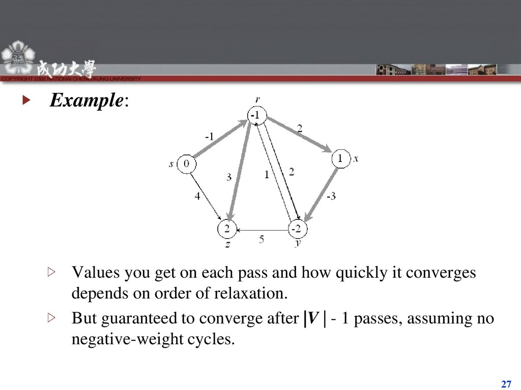
vertices. Shaded edges show shortest paths.] This example shows that the shortest path might not be unique. It also shows that when we look at shortest paths from one vertex to all other vertices, the shortest paths are organized as tree.
accumulates linearly along a path. we want to minimize. Example: time, cost, penalties, loss. Generalization of breadth-first search to weighted graphs.
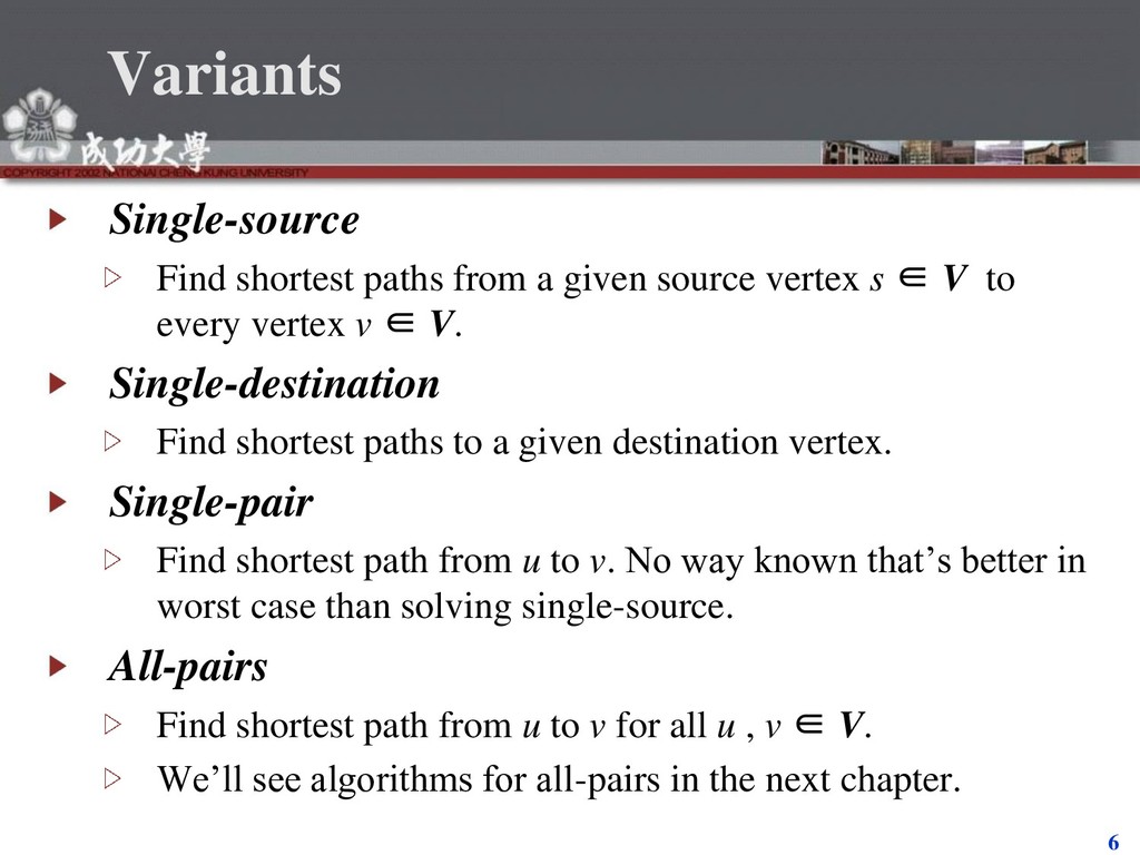
vertex s ∈ V to every vertex v ∈ V. Single-destination Find shortest paths to a given destination vertex. Single-pair Find shortest path from u to v. No way known that’s better in worst case than solving single-source. All-pairs Find shortest path from u to v for all u , v ∈ V. We’ll see algorithms for all-pairs in the next chapter.
are reachable from the source. If we have a negative-weight cycle, we can just keep going around it, and get w(s, v) = -∞ for all v on the cycle. But OK if the negative-weight cycle is not reachable from the source. Some algorithms work only if there are no negative-weight edges in the graph. We’ll be clear when they’re allowed and not allowed.
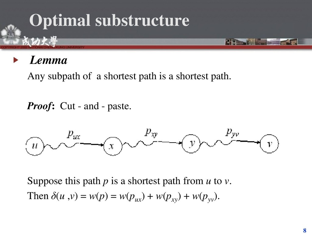
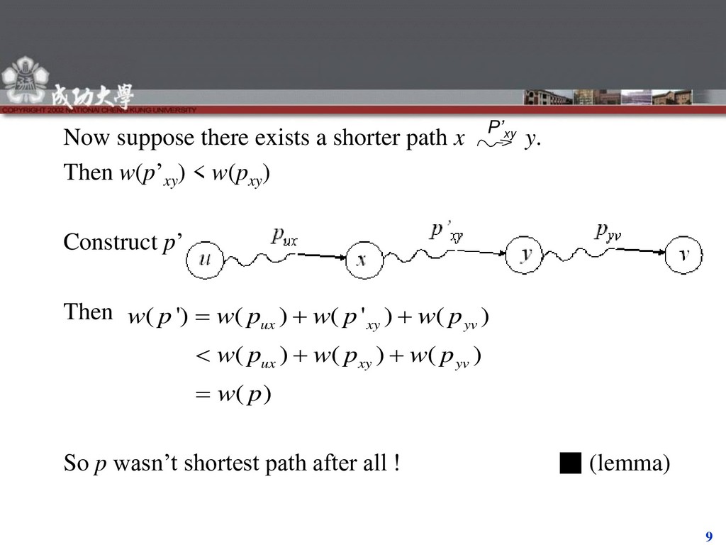
Then w(p’xy ) < w(pxy ) Construct p’ : Then So p wasn’t shortest path after all ! ▪ (lemma) P’xy ( ') ( ) ( ' ) ( ) ( ) ( ) ( ) ( ) ux xy yv ux xy yv w p w p w p w p w p w p w p w p
out negative-weight cycles. Positive-weight ⇒ we can get a shorter path by omitting the cycle. Zero-weight: no reason to use them ⇒ assume that our solutions won’t use them.
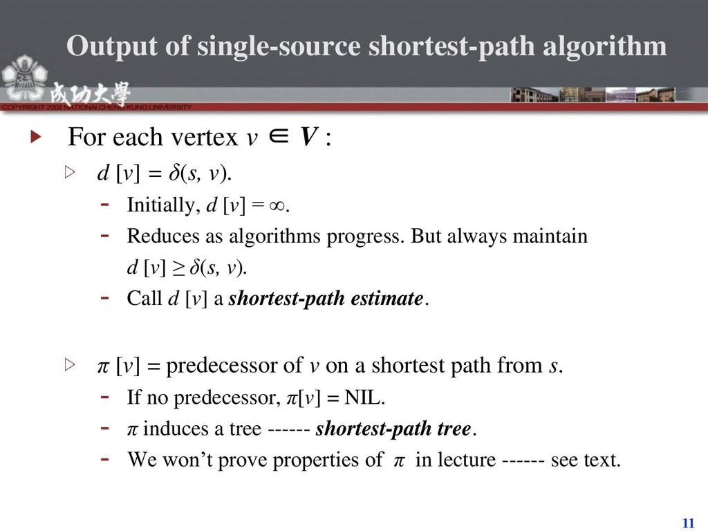
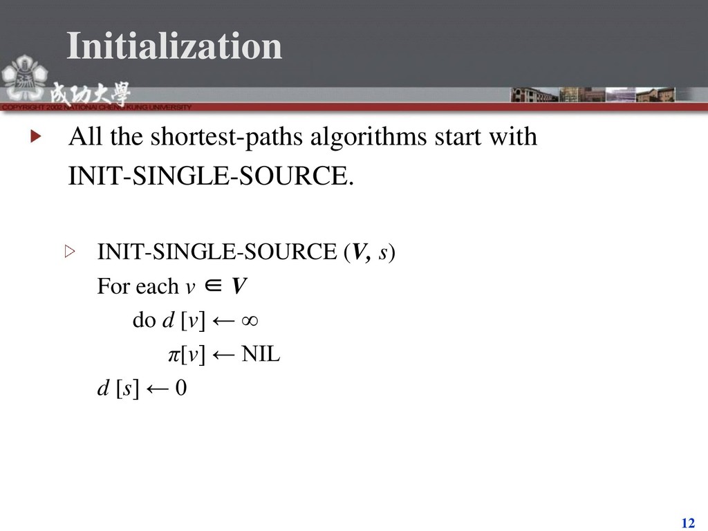
∈ V : d [v] = δ(s, v). Initially, d [v] = ∞. Reduces as algorithms progress. But always maintain d [v] ≥ δ(s, v). Call d [v] a shortest-path estimate. π [v] = predecessor of v on a shortest path from s. If no predecessor, π[v] = NIL. π induces a tree ------ shortest-path tree. We won’t prove properties of π in lecture ------ see text.
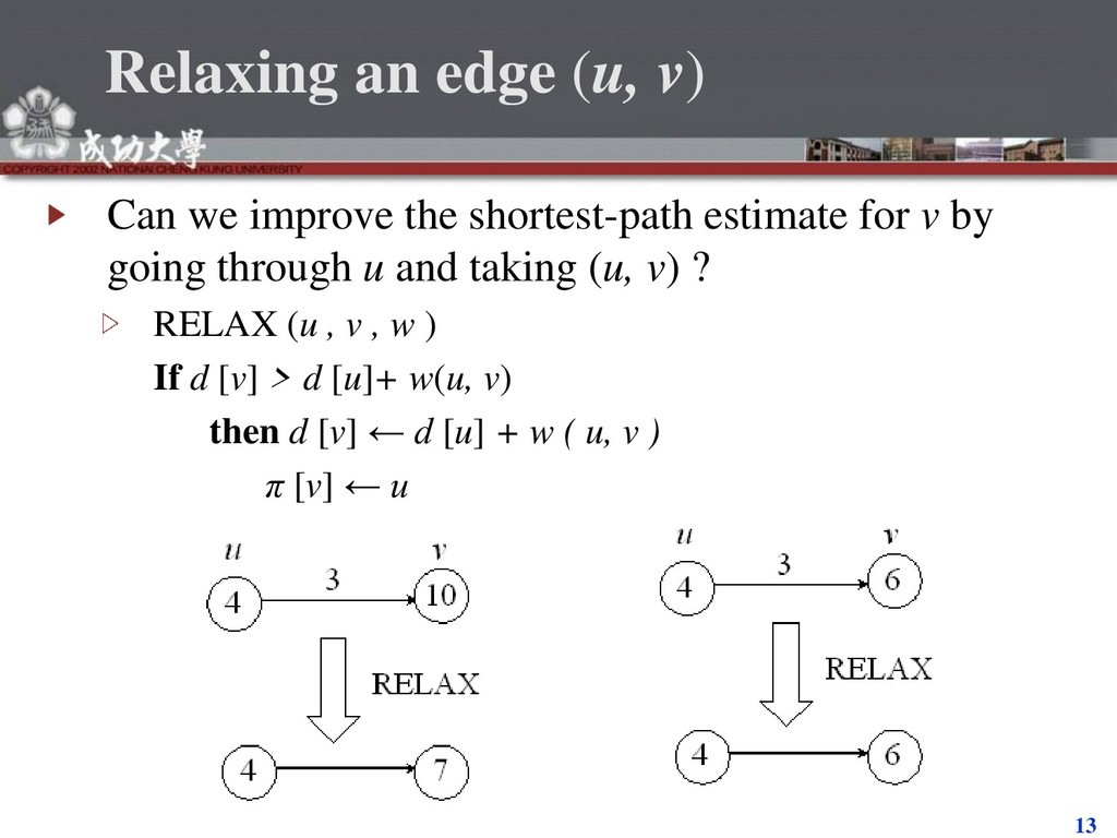
shortest-path estimate for v by going through u and taking (u, v) ? RELAX (u , v , w ) If d [v] > d [u]+ w(u, v) then d [v] ← d [u] + w ( u, v ) π [v] ← u
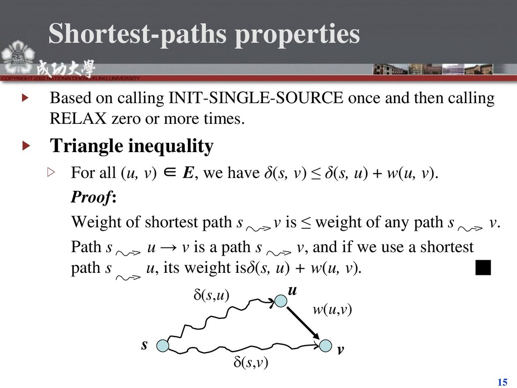
calling RELAX zero or more times. Triangle inequality For all (u, v) ∈ E, we have δ(s, v) ≤ δ(s, u) + w(u, v). Proof: Weight of shortest path s v is ≤ weight of any path s v. Path s u → v is a path s v, and if we use a shortest path s u, its weight isδ(s, u) + w(u, v). ▪ s u v w(u,v) (s,u) (s,v)
for all v. Once d [v] = δ(s, v), it never changes. Proof: Initially true. Suppose there exists a vertex such that d [v] < δ(s, v). Without loss of generality, v is first vertex for which this happens. Let u be the vertex that causes d [v] to change. Then d [v] = d [u] + w(u, v). So, d [v] < δ(s, v) ≤ δ(s, u) + w(u, v) (triangle inequality) ≤ d [u] + w(u, v) (v is first violation) ⇒ d [v] < d [u] + w(u, v). (Contradicts d [v] = d [u] + w(u, v)) Once d [v] reaches δ(s, v), it never goes lower. It never goes up, since relaxations only lower shortest-path estimates. ▪
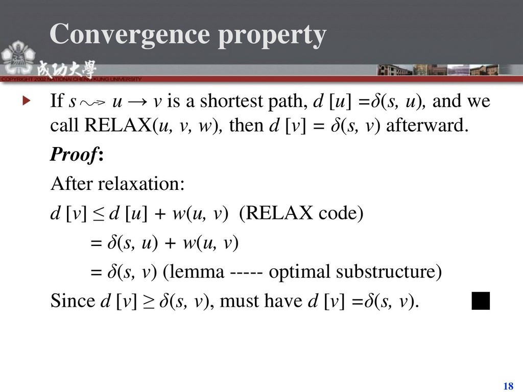
shortest path, d [u] =δ(s, u), and we call RELAX(u, v, w), then d [v] = δ(s, v) afterward. Proof: After relaxation: d [v] ≤ d [u] + w(u, v) (RELAX code) = δ(s, u) + w(u, v) = δ(s, v) (lemma ----- optimal substructure) Since d [v] ≥ δ(s, v), must have d [v] =δ(s, v). ▪
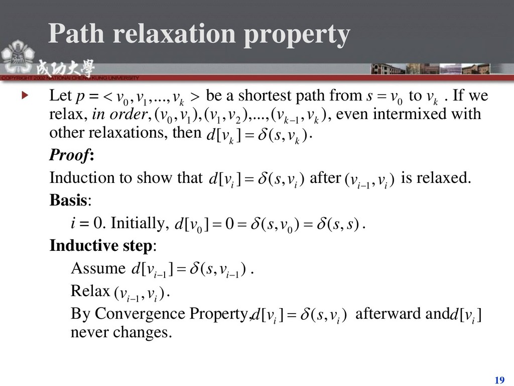
path from . If we relax, in order, , even intermixed with other relaxations, then . Proof: Induction to show that after is relaxed. Basis: i = 0. Initially, . Inductive step: Assume . Relax . By Convergence Property, afterward and never changes. 0 1 , ,..., k v v v 0 to k s v v ) , ( ),..., , ( ), , ( 1 2 1 1 0 k k v v v v v v [ ] ( , ) k k d v s v [ ] ( , ) i i d v s v 1 ( , ) i i v v 0 0 [ ] 0 ( , ) ( , ) d v s v s s 1 1 [ ] ( , ) i i d v s v 1 ( , ) i i v v [ ] ( , ) i i d v s v [ ] i d v
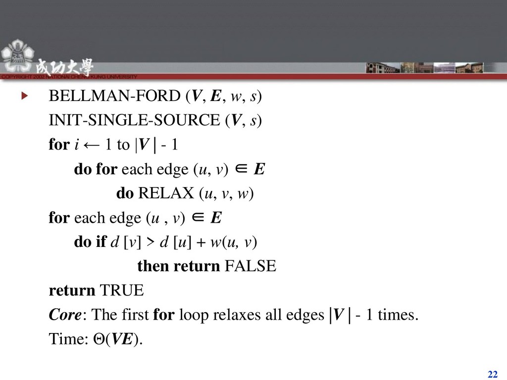
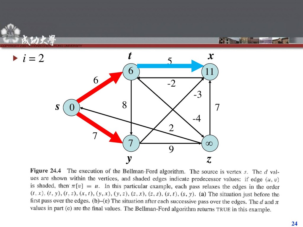
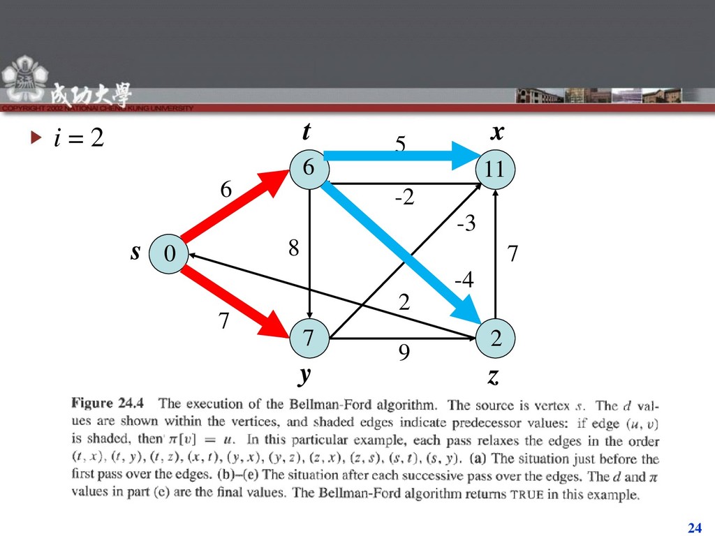
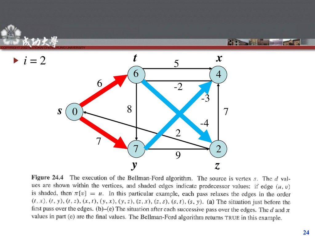
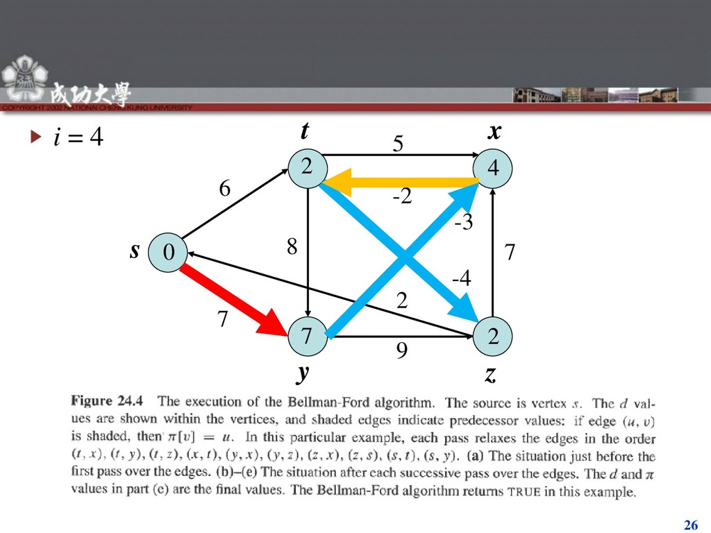
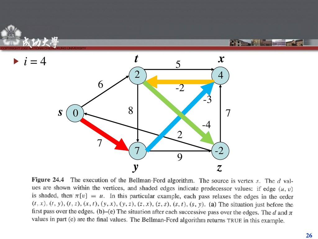
i ← 1 to |V | - 1 do for each edge (u, v) ∈ E do RELAX (u, v, w) for each edge (u , v) ∈ E do if d [v] > d [u] + w(u, v) then return FALSE return TRUE Core: The first for loop relaxes all edges |V | - 1 times. Time: Θ(VE).
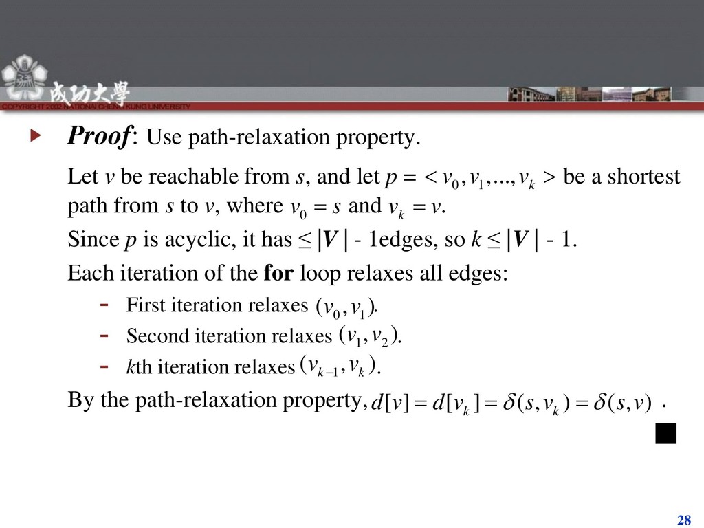
s, and let p = be a shortest path from s to v, where and . Since p is acyclic, it has ≤ |V | - 1edges, so k ≤ |V | - 1. Each iteration of the for loop relaxes all edges: First iteration relaxes . Second iteration relaxes . kth iteration relaxes . By the path-relaxation property, . ▪ 0 1 , ,..., k v v v 0 v s k v v 0 1 ( , ) v v 1 2 ( , ) v v 1 ( , ) k k v v [ ] [ ] ( , ) ( , ) k k d v d v s v s v
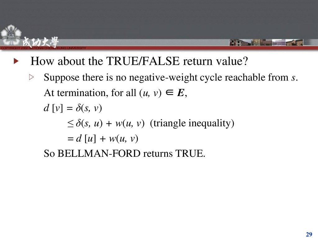
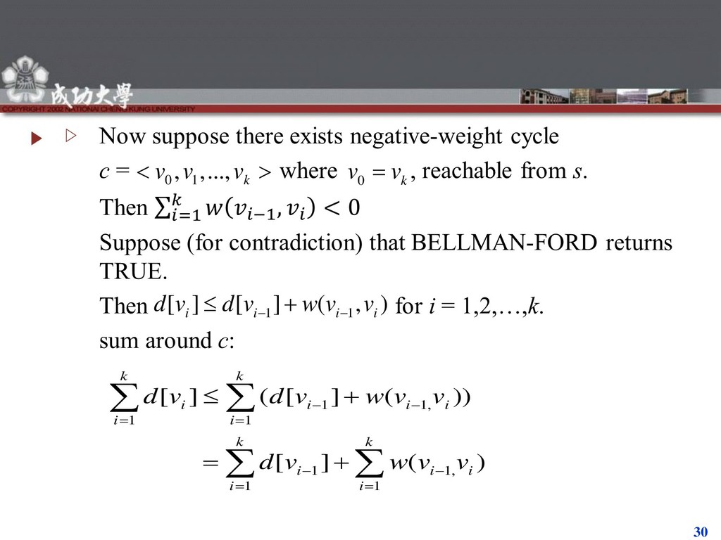
no negative-weight cycle reachable from s. At termination, for all (u, v) ∈ E, d [v] = δ(s, v) ≤ δ(s, u) + w(u, v) (triangle inequality) = d [u] + w(u, v) So BELLMAN-FORD returns TRUE.
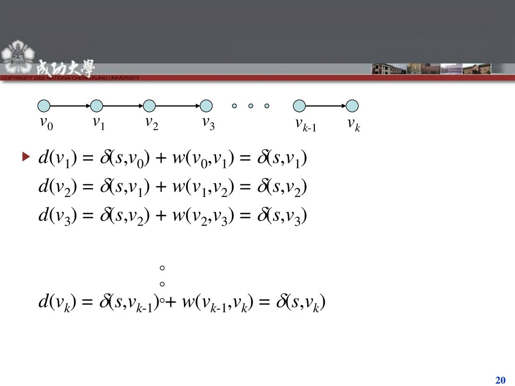
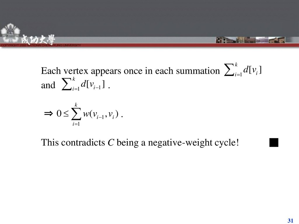
0 k v v 1 1, 1 1 1 1, 1 1 [ ] ( [ ] ( )) [ ] ( ) k k i i i i i i k k i i i i i d v d v w v v d v w v v 1 1 [ ] [ ] ( , ) i i i i d v d v w v v
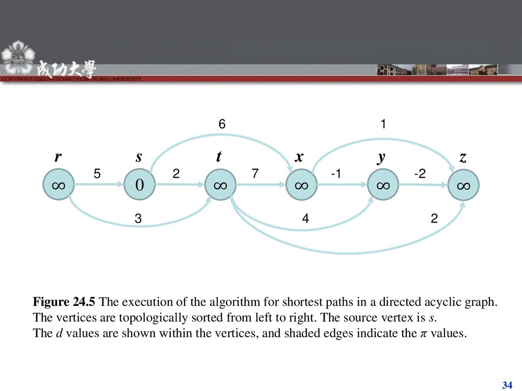
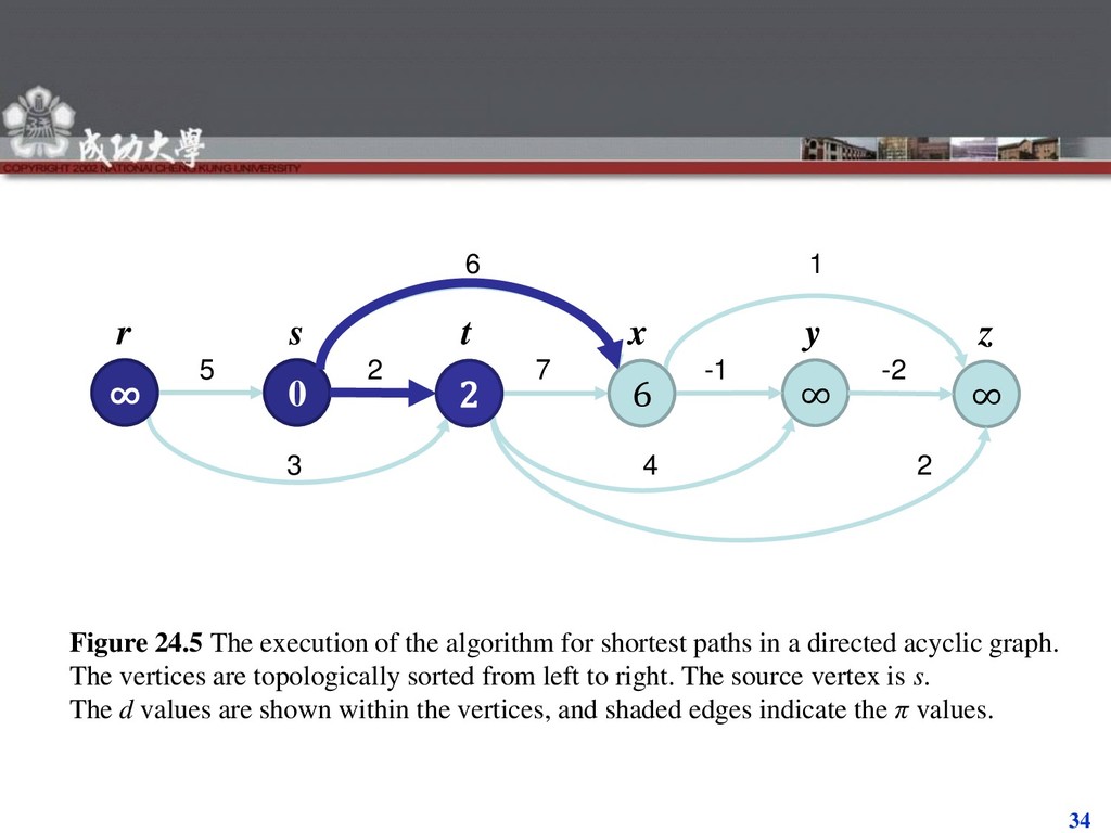
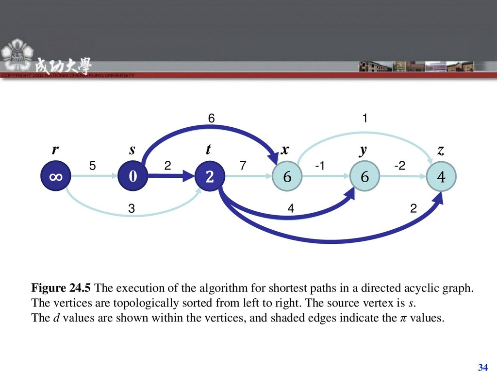
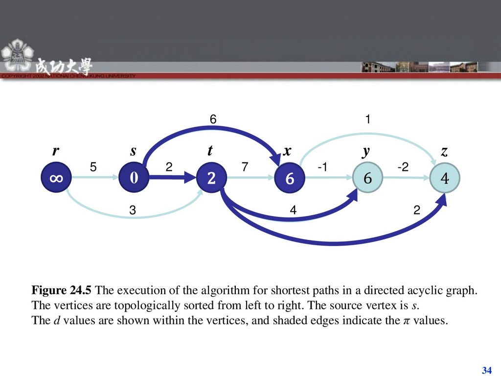
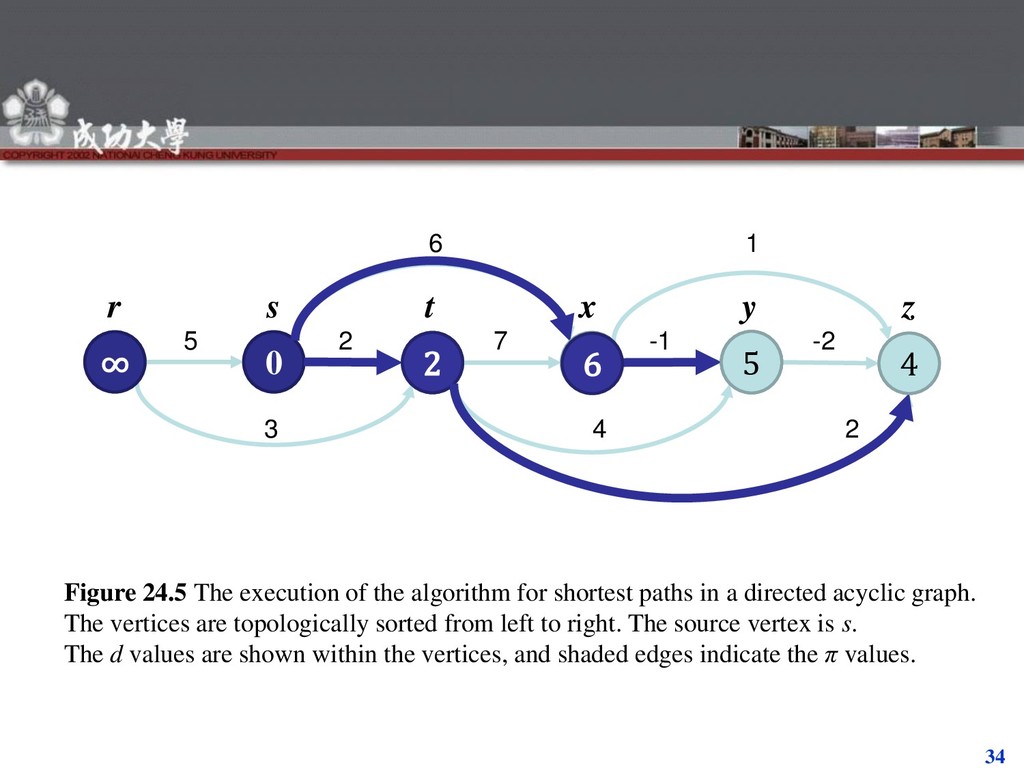
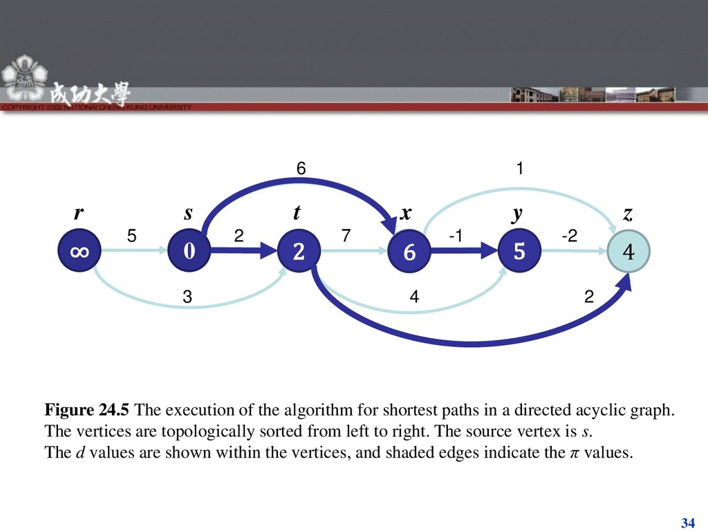
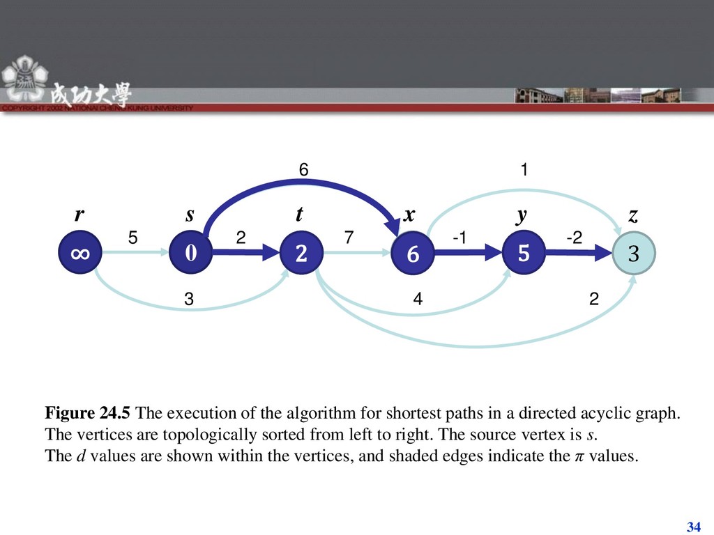
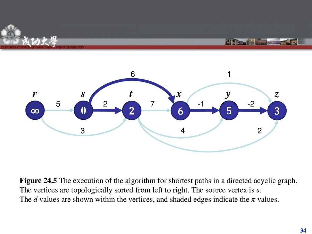
a dag, we’re guaranteed no negative-weight cycles. DAG-SHORTEST-PATHS (V, E, w, s) topologically sort the vertices INIT-SINGLE-SOURCE (V, s) for each vertex u, taken in topologically sorted order do for each vertex v ∈ Adj [u] do RELAX (u, v, w)
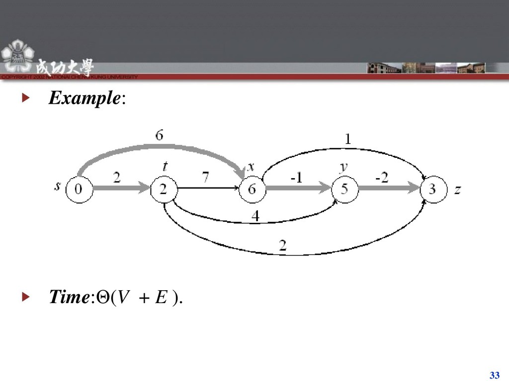
-1 -2 6 1 3 4 2 r s t x y z Figure 24.5 The execution of the algorithm for shortest paths in a directed acyclic graph. The vertices are topologically sorted from left to right. The source vertex is s. The d values are shown within the vertices, and shaded edges indicate the π values.
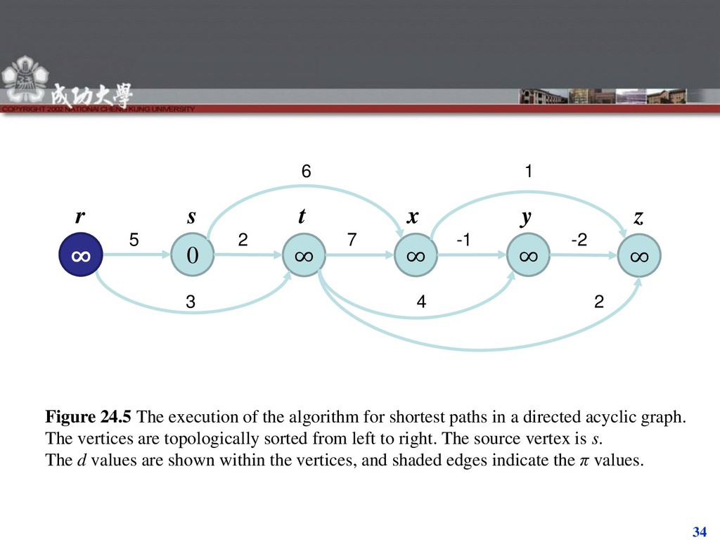
-1 -2 6 1 3 4 2 ∞ r s t x y z Figure 24.5 The execution of the algorithm for shortest paths in a directed acyclic graph. The vertices are topologically sorted from left to right. The source vertex is s. The d values are shown within the vertices, and shaded edges indicate the π values.
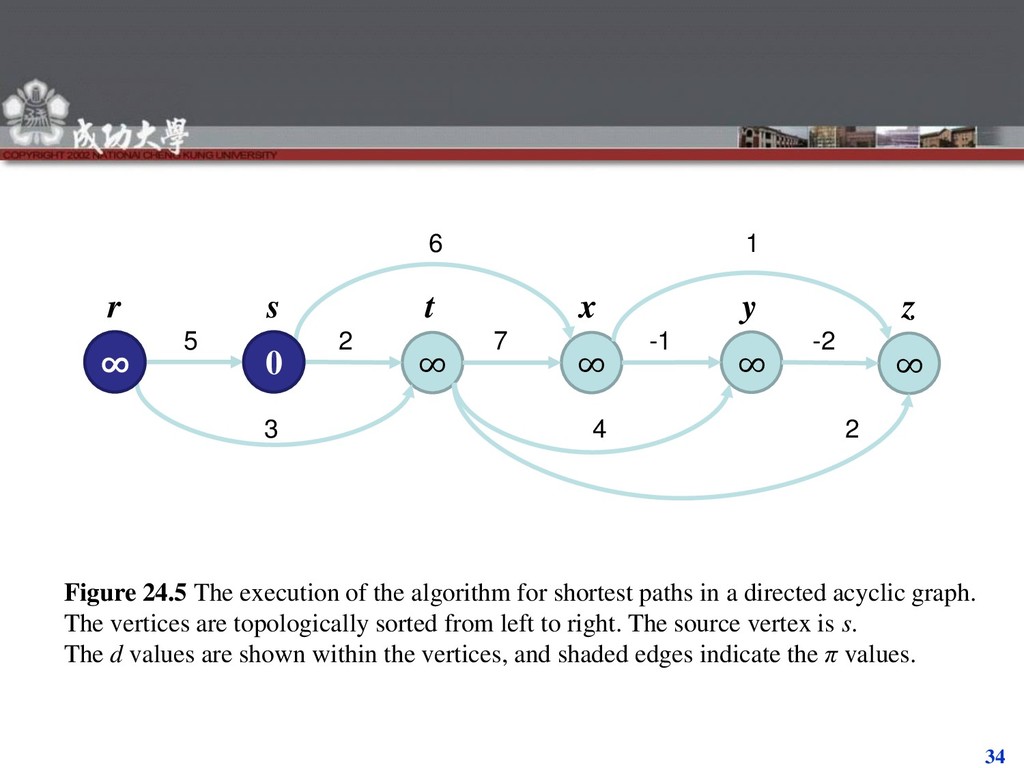
-1 -2 6 1 3 4 2 ∞ r s t x y z 0 Figure 24.5 The execution of the algorithm for shortest paths in a directed acyclic graph. The vertices are topologically sorted from left to right. The source vertex is s. The d values are shown within the vertices, and shaded edges indicate the π values.
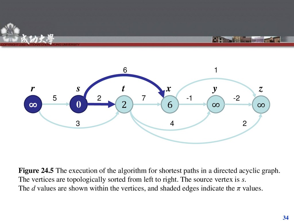
-1 -2 6 1 3 4 2 ∞ r s t x y z 0 6 2 Figure 24.5 The execution of the algorithm for shortest paths in a directed acyclic graph. The vertices are topologically sorted from left to right. The source vertex is s. The d values are shown within the vertices, and shaded edges indicate the π values.
-1 -2 6 1 3 4 2 ∞ r s t x y z 0 6 2 2 Figure 24.5 The execution of the algorithm for shortest paths in a directed acyclic graph. The vertices are topologically sorted from left to right. The source vertex is s. The d values are shown within the vertices, and shaded edges indicate the π values.
-1 -2 6 1 3 4 2 ∞ r s t x y z 0 6 2 2 6 4 Figure 24.5 The execution of the algorithm for shortest paths in a directed acyclic graph. The vertices are topologically sorted from left to right. The source vertex is s. The d values are shown within the vertices, and shaded edges indicate the π values.
-1 -2 6 1 3 4 2 ∞ r s t x y z 0 6 2 2 6 4 6 Figure 24.5 The execution of the algorithm for shortest paths in a directed acyclic graph. The vertices are topologically sorted from left to right. The source vertex is s. The d values are shown within the vertices, and shaded edges indicate the π values.
-1 -2 6 1 3 4 2 ∞ r s t x y z 0 6 2 2 6 4 6 5 Figure 24.5 The execution of the algorithm for shortest paths in a directed acyclic graph. The vertices are topologically sorted from left to right. The source vertex is s. The d values are shown within the vertices, and shaded edges indicate the π values.
-1 -2 6 1 3 4 2 ∞ r s t x y z 0 6 2 2 6 4 6 5 5 Figure 24.5 The execution of the algorithm for shortest paths in a directed acyclic graph. The vertices are topologically sorted from left to right. The source vertex is s. The d values are shown within the vertices, and shaded edges indicate the π values.
-1 -2 6 1 3 4 2 ∞ r s t x y z 0 6 2 2 6 4 6 5 5 3 Figure 24.5 The execution of the algorithm for shortest paths in a directed acyclic graph. The vertices are topologically sorted from left to right. The source vertex is s. The d values are shown within the vertices, and shaded edges indicate the π values.
-1 -2 6 1 3 4 2 ∞ r s t x y z 0 6 2 2 6 4 6 5 5 3 3 Figure 24.5 The execution of the algorithm for shortest paths in a directed acyclic graph. The vertices are topologically sorted from left to right. The source vertex is s. The d values are shown within the vertices, and shaded edges indicate the π values.
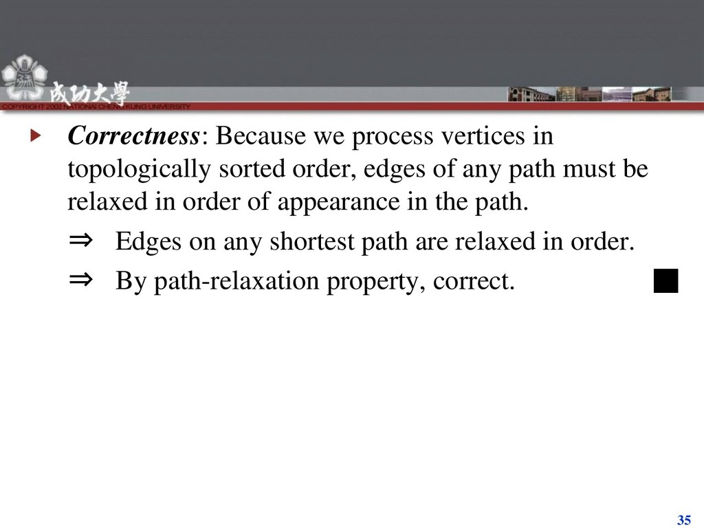
edges of any path must be relaxed in order of appearance in the path. ⇒ Edges on any shortest path are relaxed in order. ⇒ By path-relaxation property, correct. ▪
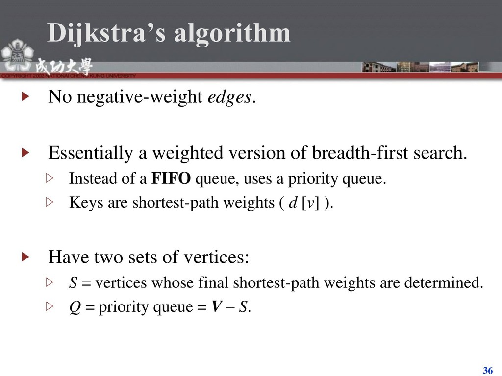
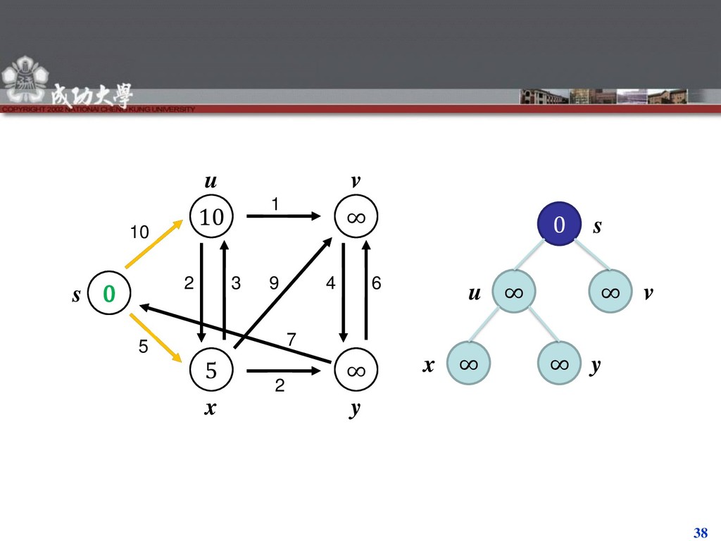
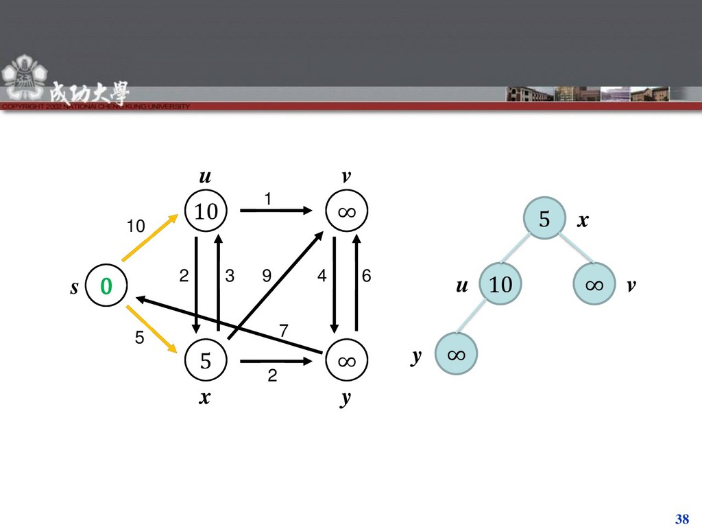
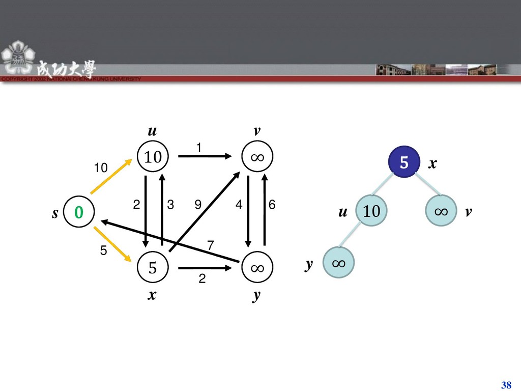
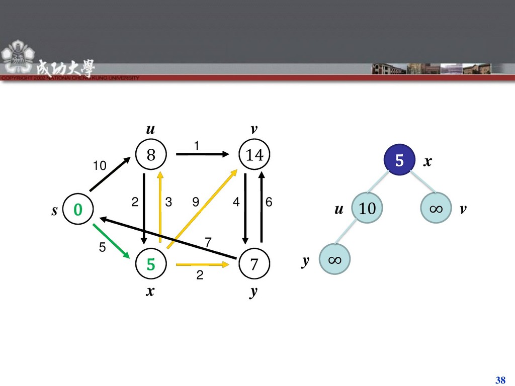
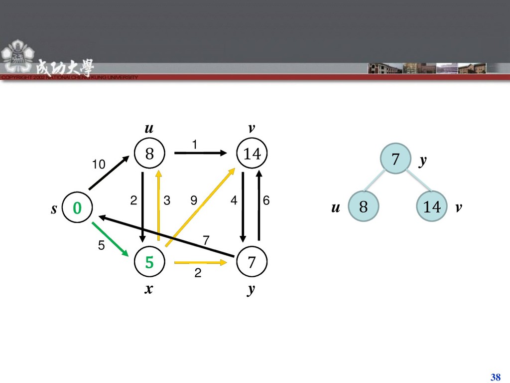
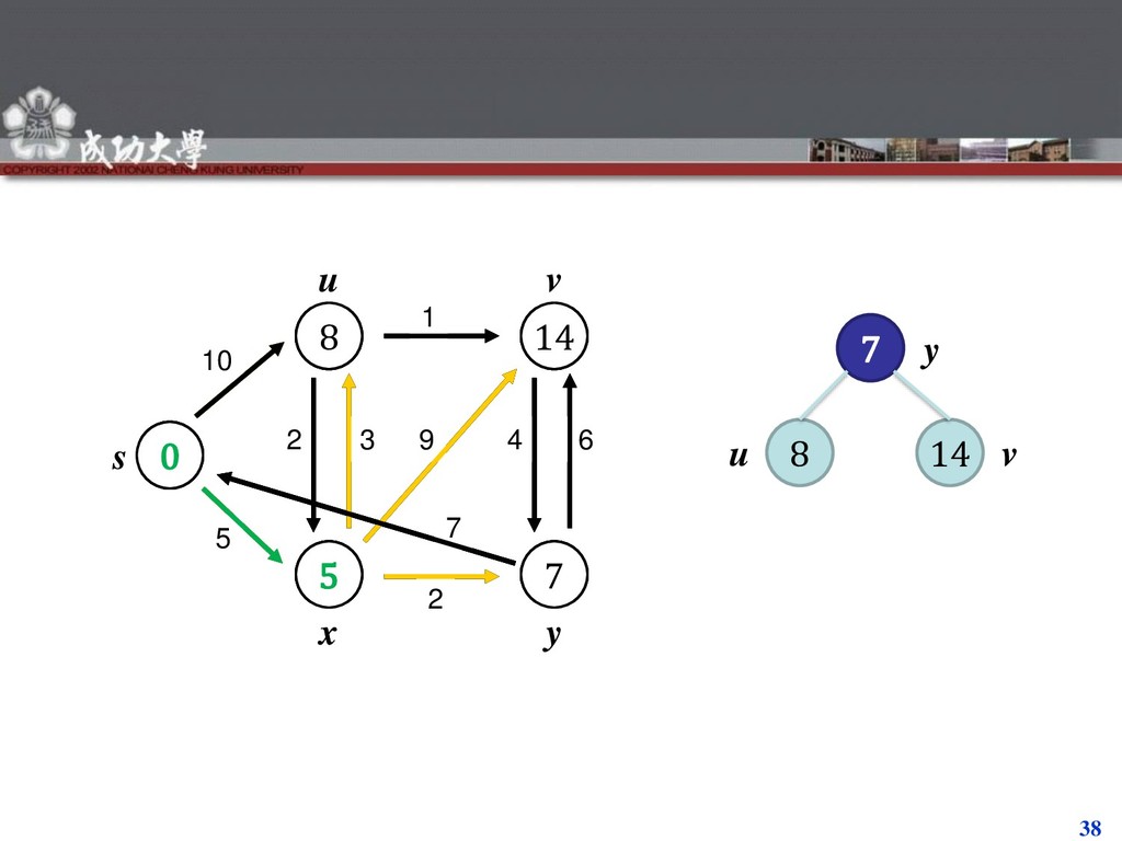
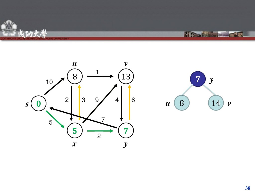
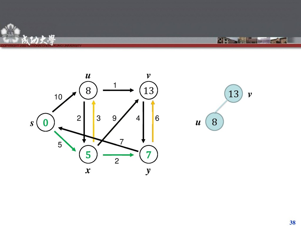
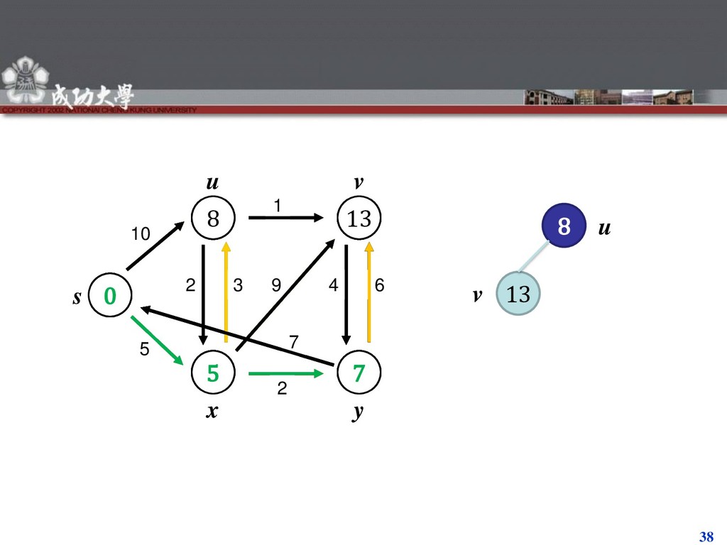
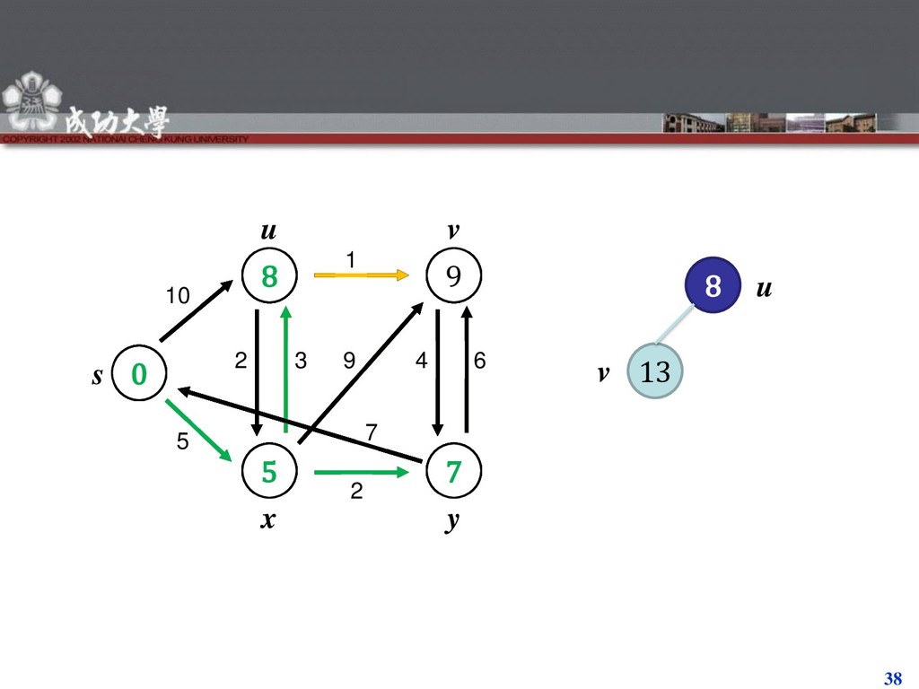
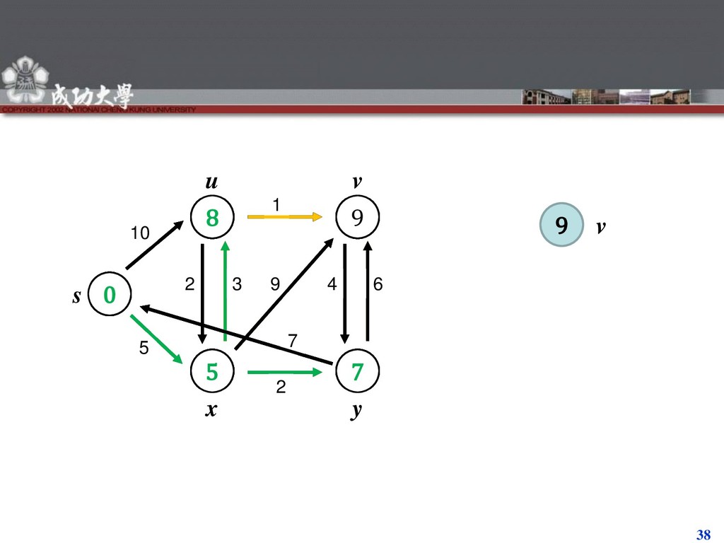
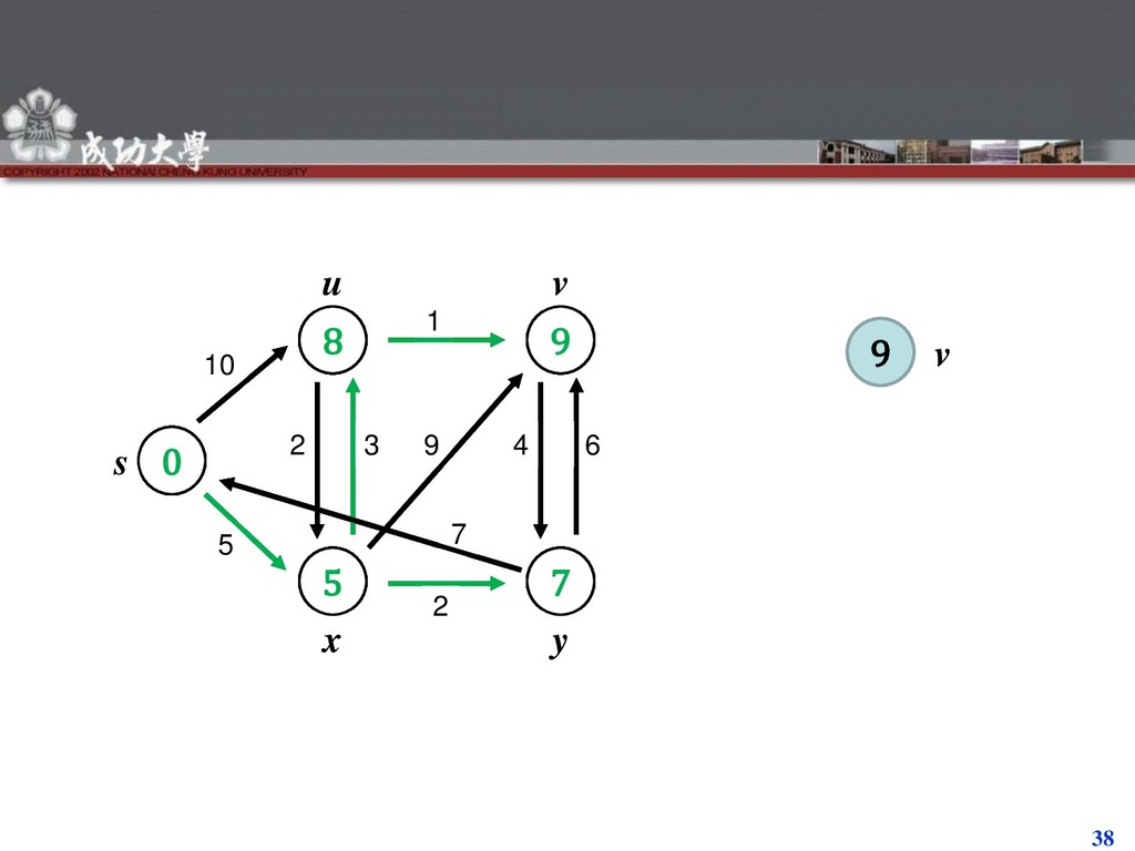
of breadth-first search. Instead of a FIFO queue, uses a priority queue. Keys are shortest-path weights ( d [v] ). Have two sets of vertices: S = vertices whose final shortest-path weights are determined. Q = priority queue = V – S.
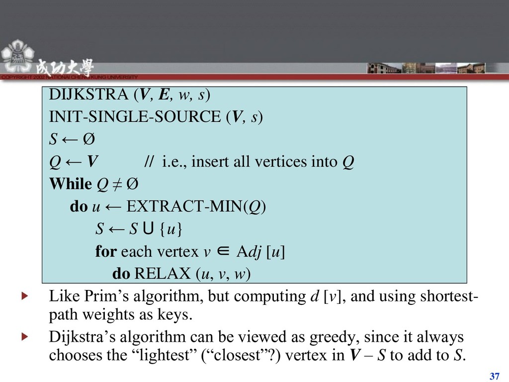
← Ø Q ← V // i.e., insert all vertices into Q While Q ≠ Ø do u ← EXTRACT-MIN(Q) S ← S U {u} for each vertex v ∈ Adj [u] do RELAX (u, v, w) Like Prim’s algorithm, but computing d [v], and using shortest- path weights as keys. Dijkstra’s algorithm can be viewed as greedy, since it always chooses the “lightest” (“closest”?) vertex in V – S to add to S.
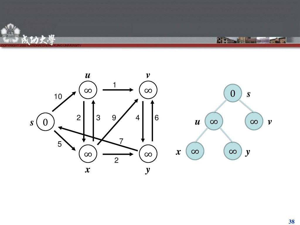
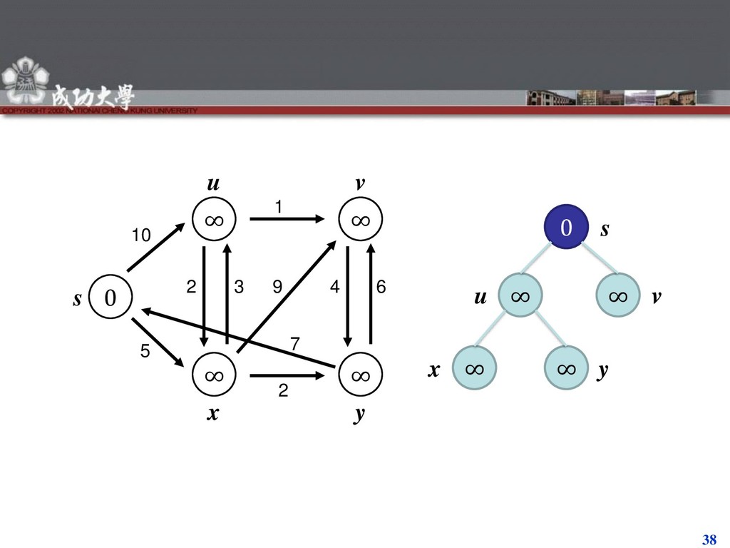
7 s x y u v ∞ ∞ ∞ ∞ 0 10 1 5 2 3 2 4 6 9 7 s x y u v 10 ∞ ∞ 5 0 10 1 5 2 3 2 4 6 9 7 s x y u v 8 7 14 5 0 14 8 7 y u v y 10 1 5 2 3 2 4 6 9 7 s x y u v 8 7 13 5 0
7 s x y u v ∞ ∞ ∞ ∞ 0 10 1 5 2 3 2 4 6 9 7 s x y u v 10 ∞ ∞ 5 0 10 1 5 2 3 2 4 6 9 7 s x y u v 8 7 14 5 0 10 1 5 2 3 2 4 6 9 7 s x y u v 8 7 13 5 0 8 13 v u v y
7 s x y u v ∞ ∞ ∞ ∞ 0 10 1 5 2 3 2 4 6 9 7 s x y u v 10 ∞ ∞ 5 0 10 1 5 2 3 2 4 6 9 7 s x y u v 8 7 14 5 0 10 1 5 2 3 2 4 6 9 7 s x y u v 8 7 13 5 0 13 8 u v v y
7 s x y u v ∞ ∞ ∞ ∞ 0 10 1 5 2 3 2 4 6 9 7 s x y u v 10 ∞ ∞ 5 0 10 1 5 2 3 2 4 6 9 7 s x y u v 8 7 14 5 0 10 1 5 2 3 2 4 6 9 7 s x y u v 8 7 13 5 0 13 8 u v v y
7 s x y u v ∞ ∞ ∞ ∞ 0 10 1 5 2 3 2 4 6 9 7 s x y u v 10 ∞ ∞ 5 0 10 1 5 2 3 2 4 6 9 7 s x y u v 8 7 14 5 0 10 1 5 2 3 2 4 6 9 7 s x y u v 8 7 13 5 0 13 8 u v v y 10 1 5 2 3 2 4 6 9 7 s x y u v 8 7 9 5 0
7 s x y u v ∞ ∞ ∞ ∞ 0 10 1 5 2 3 2 4 6 9 7 s x y u v 10 ∞ ∞ 5 0 10 1 5 2 3 2 4 6 9 7 s x y u v 8 7 14 5 0 10 1 5 2 3 2 4 6 9 7 s x y u v 8 7 13 5 0 10 1 5 2 3 2 4 6 9 7 s x y u v 8 7 9 5 0 9 v v y
7 s x y u v ∞ ∞ ∞ ∞ 0 10 1 5 2 3 2 4 6 9 7 s x y u v 10 ∞ ∞ 5 0 10 1 5 2 3 2 4 6 9 7 s x y u v 8 7 14 5 0 10 1 5 2 3 2 4 6 9 7 s x y u v 8 7 13 5 0 10 1 5 2 3 2 4 6 9 7 s x y u v 8 7 9 5 0 9 v v y 10 1 5 2 3 2 4 6 9 7 s x y u v 8 7 9 5 0
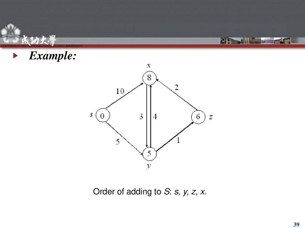
iteration of the while loop, d [v] = δ(s, v) for all v ∈ S. Initialization: Initially, S = Ø , so trivially true. Termination: At end, Q= Ø ⇒ S = V ⇒ d [v] = δ(s, v) for all v ∈ V.
u) when u is added to S in each iteration. Suppose there exists u such that d [u] ≠ δ(s, u). Without loss of generality, let u be the first vertex for which d [u] ≠ δ(s, u) when u is added to S. Observations: u ≠ s, since d [s] = δ(s, s) = 0. Therefore, s ∈ S , so S ≠ Ø . There must be some path s u, since otherwise d [u]= δ(s, u) = ∞ by no-path property.
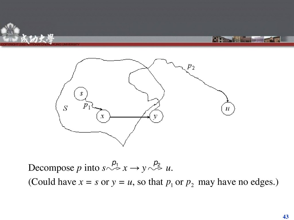
a shortest path s u. Just before u is added to S, path p connects a vertex in S ( i.e., s ) to a vertex in V - S ( i.e., u ). Let y be first vertex along p that’s in V - S, and let x ∈ S be y’s predecessor. p
added to S. Proof x ∈ S and u is the first vertex such that d [u] ≠ δ(s, u) when u is added to S ⇒ d [x] = δ(s, x) when x is added to S. Relaxed (x , y) at that time, so by the convergence property, d [y] = δ(s, y). ▪ (claim)
δ(s, u): y is on shortest path s u, and all edge weights are nonnegative ⇒ δ(s, y) ≤ δ(s, u) ⇒ d [y] = δ(s, y) ≤ δ(s, u) ≤ d [u] (upper-bound property). Also, both y and u were in Q when we chose u, so d [u] ≤ d [y] ⇒ d [u] = d [y]. Therefore, d [y] = δ(s, y) = δ(s, u) = d [u]. Contradicts assumption that d [u] ≠ δ(s, u). Hence, Dijkstra’s algorithm is correct. ▪
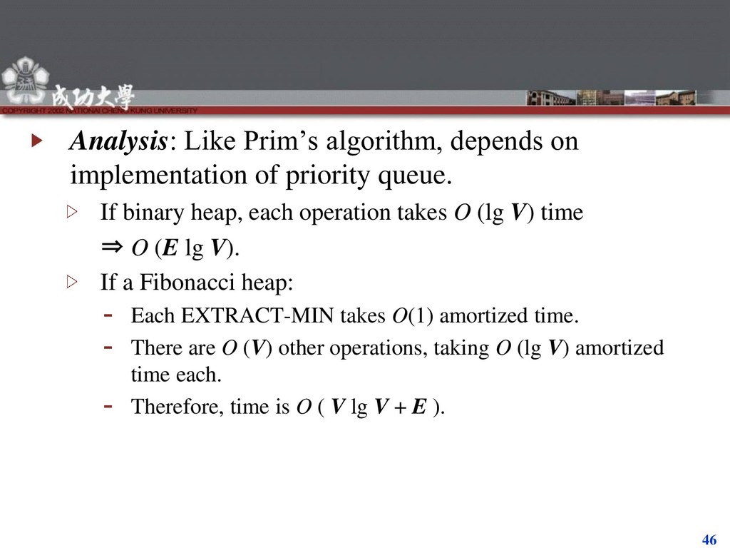
queue. If binary heap, each operation takes O (lg V) time ⇒ O (E lg V). If a Fibonacci heap: Each EXTRACT-MIN takes O(1) amortized time. There are O (V) other operations, taking O (lg V) amortized time each. Therefore, time is O ( V lg V + E ).
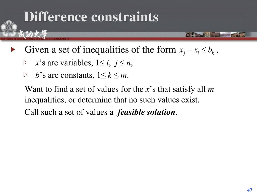
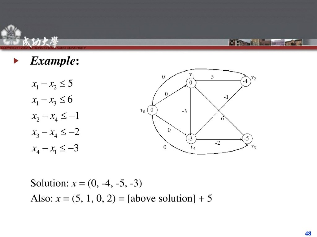
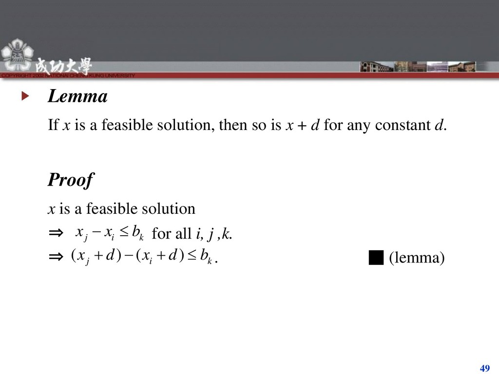
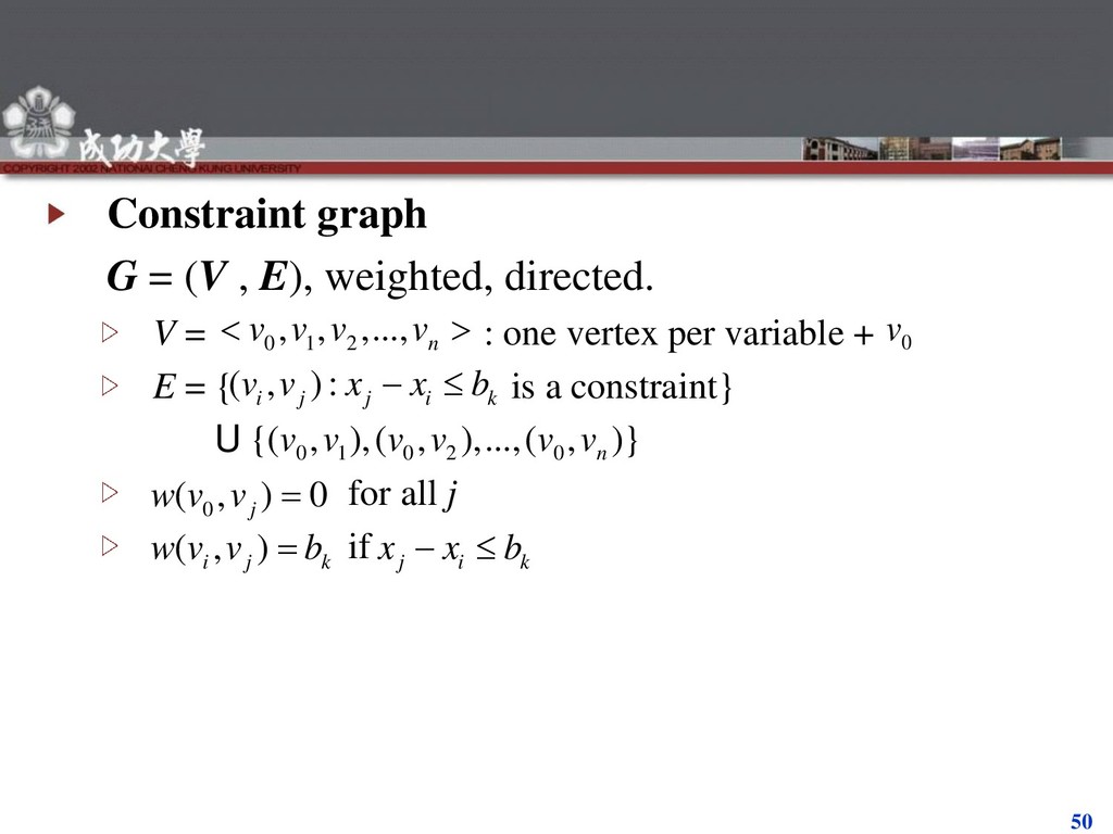
form . x’s are variables, 1≤ i, j ≤ n, b’s are constants, 1≤ k ≤ m. Want to find a set of values for the x’s that satisfy all m inequalities, or determine that no such values exist. Call such a set of values a feasible solution. j i k x x b
V = : one vertex per variable + E = { is a constraint} U for all j if 0 1 2 , , ,..., n v v v v 0 v ( , ): i j j i k v v x x b 0 1 0 2 0 {( , ),( , ),...,( , )} n v v v v v v 0 ( , ) 0 j w v v ( , ) i j k w v v b j i k x x b
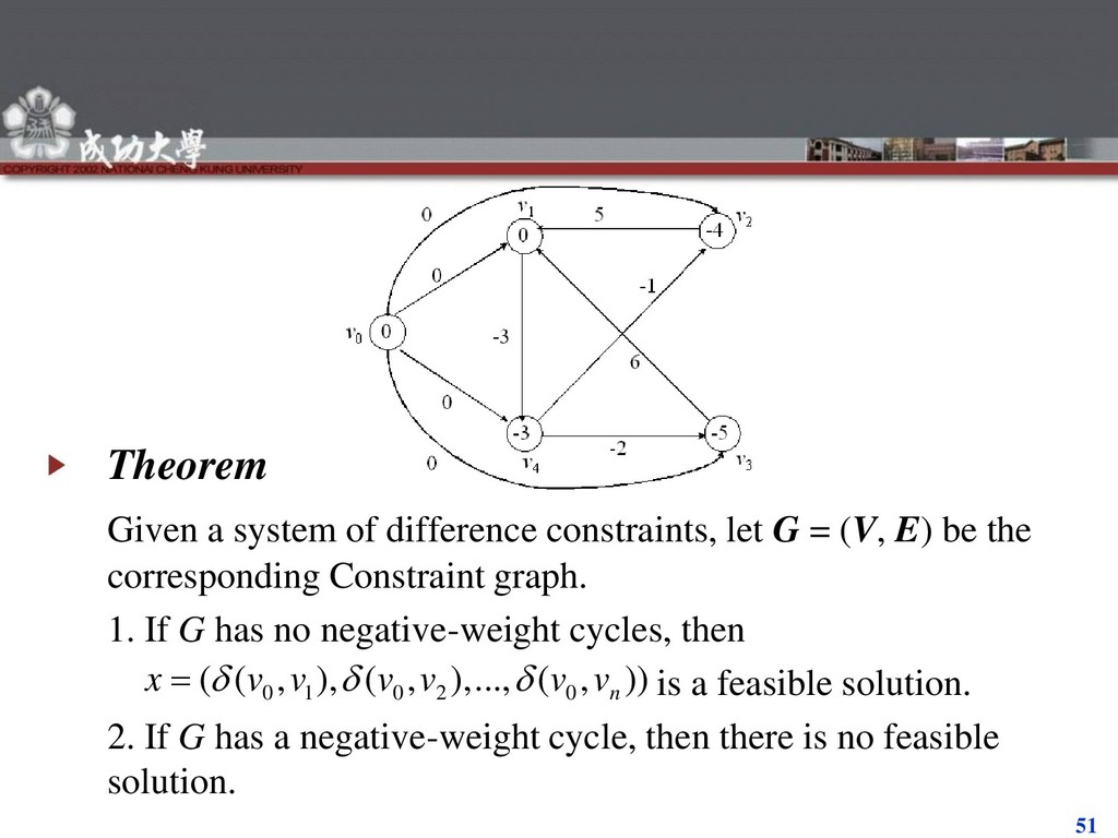
= (V, E) be the corresponding Constraint graph. 1. If G has no negative-weight cycles, then is a feasible solution. 2. If G has a negative-weight cycle, then there is no feasible solution. 0 1 0 2 0 ( ( , ), ( , ),..., ( , )) n x v v v v v v
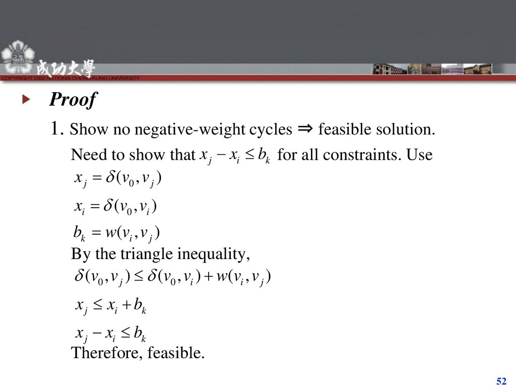
Need to show that for all constraints. Use By the triangle inequality, Therefore, feasible. j i k x x b 0 0 ( , ) ( , ) ( , ) j j i i k i j x v v x v v b w v v 0 0 ( , ) ( , ) ( , ) j i i j j i k j i k v v v v w v v x x b x x b
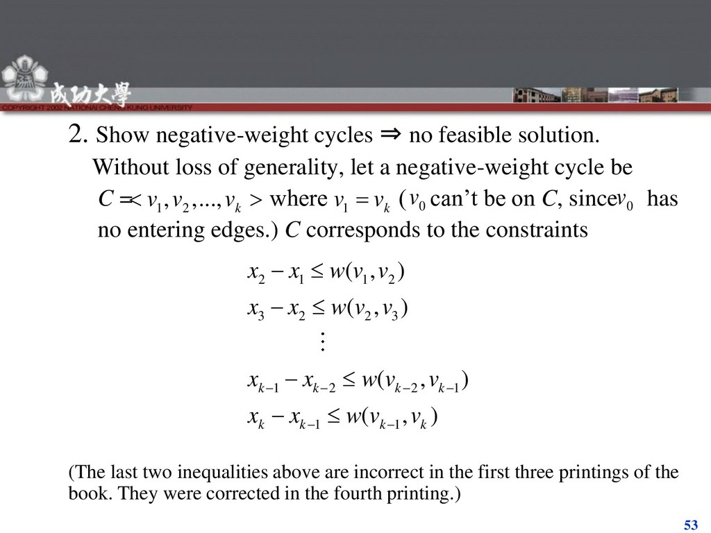
loss of generality, let a negative-weight cycle be C = where ( can’t be on C, since has no entering edges.) C corresponds to the constraints (The last two inequalities above are incorrect in the first three printings of the book. They were corrected in the fourth printing.) 2 1 1 2 3 2 2 3 1 2 2 1 1 1 ( , ) ( , ) ( , ) ( , ) k k k k k k k k x x w v v x x w v v x x w v v x x w v v 1 2 , ,..., k v v v 1 k v v 0 v 0 v
must satisfy their sum. So add them up. Each is added once and subtracted once. We get 0 ≤ w (C). But w (C) < 0 , since C is a negative-weight cycle. Contradiction ⇒ no such feasible solution x exists. ▪ (theorem) 1 1 ( ) k k v v x x i x
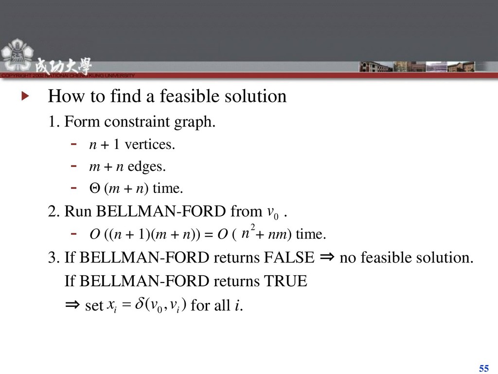
graph. n + 1 vertices. m + n edges. Θ (m + n) time. 2. Run BELLMAN-FORD from . O ((n + 1)(m + n)) = O ( + nm) time. 3. If BELLMAN-FORD returns FALSE ⇒ no feasible solution. If BELLMAN-FORD returns TRUE ⇒ set for all i. 0 v 2 n 0 ( , ) i i x v v
![16 Upper-bound property Always have d [v] ≥ δ(s, v)](https://files.speakerdeck.com/presentations/76f881224a794c6196c7e134677d917d/slide_15.jpg)
![21 The Bellman-Ford algorithm Allows negative-weight edges. Computes d [v]](https://files.speakerdeck.com/presentations/76f881224a794c6196c7e134677d917d/slide_20.jpg)
![41 Maintenance: Need to show that d [u] = δ(s,](https://files.speakerdeck.com/presentations/76f881224a794c6196c7e134677d917d/slide_106.jpg)
![44 Claim d [y] = δ(s, y) when u is](https://files.speakerdeck.com/presentations/76f881224a794c6196c7e134677d917d/slide_109.jpg)
![45 Now can get a contradiction to d [u] ≠](https://files.speakerdeck.com/presentations/76f881224a794c6196c7e134677d917d/slide_110.jpg)