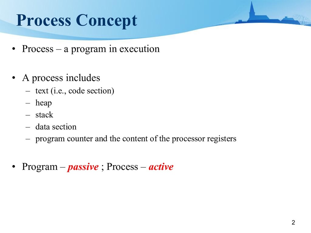
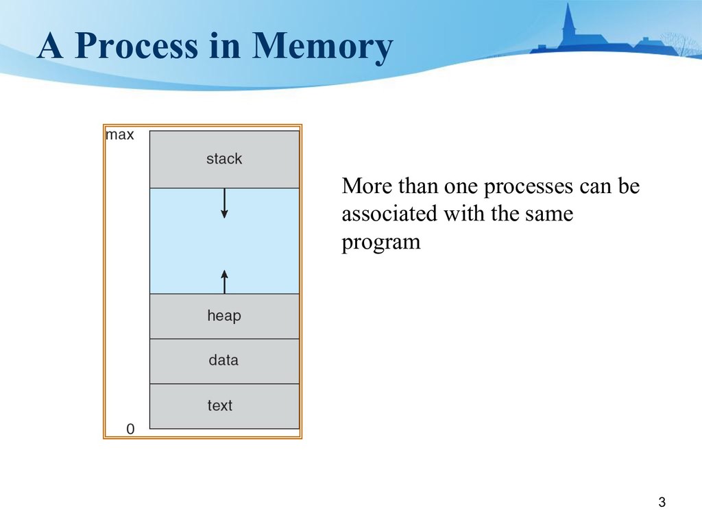
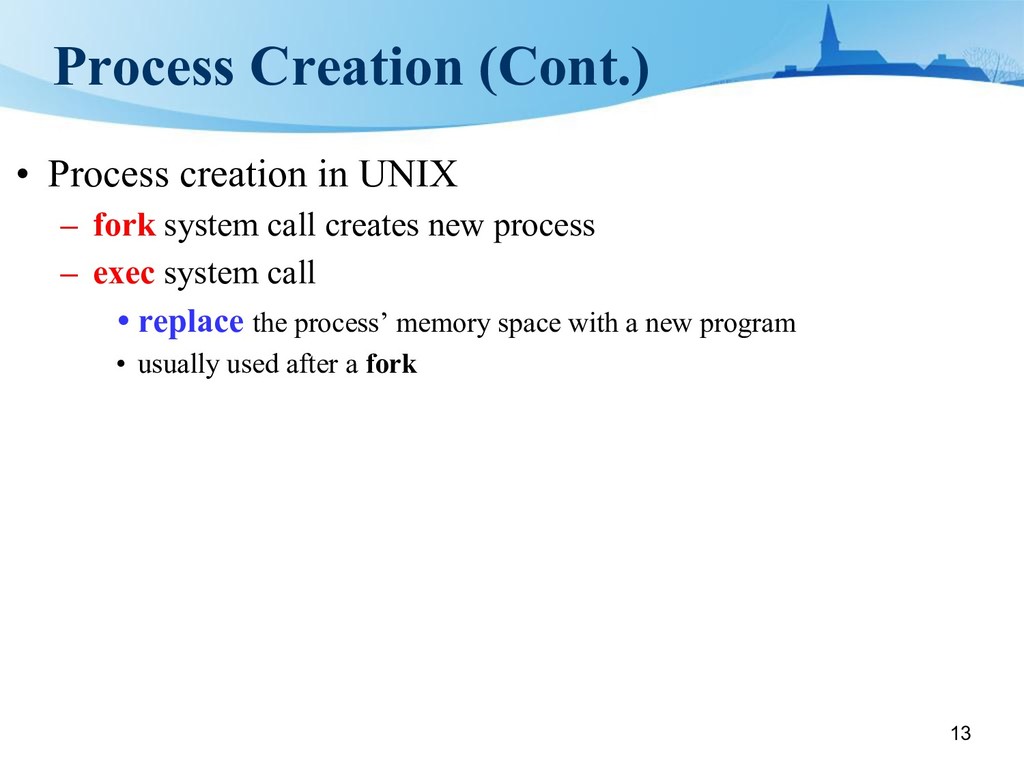
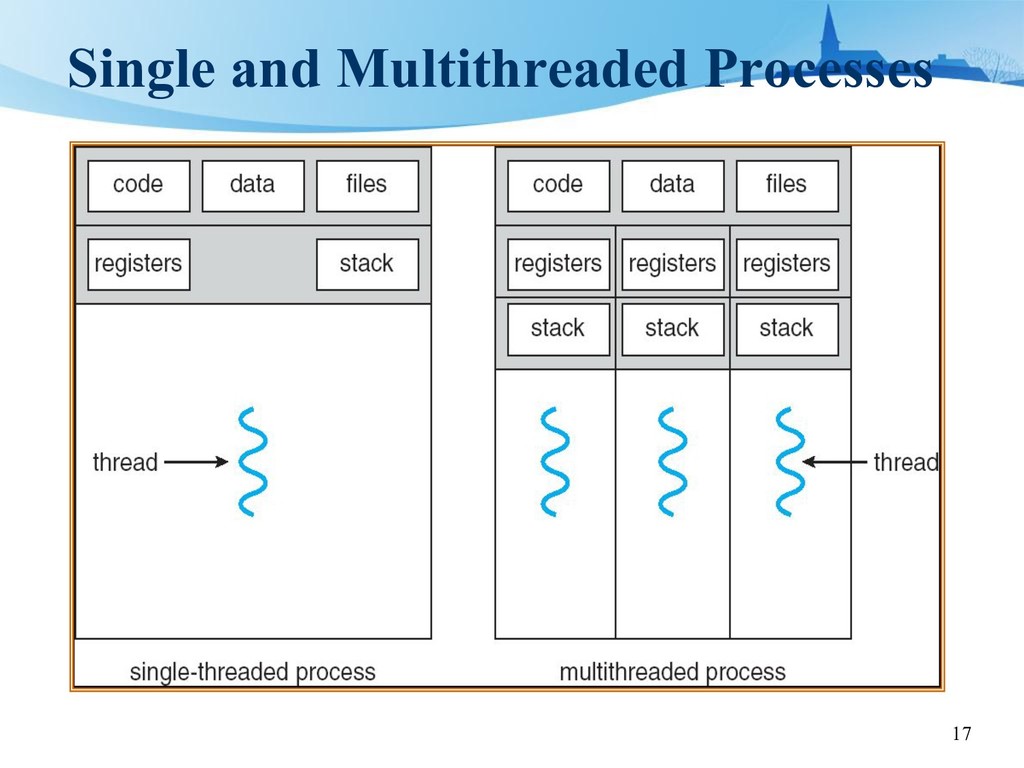
• A process includes – text (i.e., code section) – heap – stack – data section – program counter and the content of the processor registers • Program – passive ; Process – active
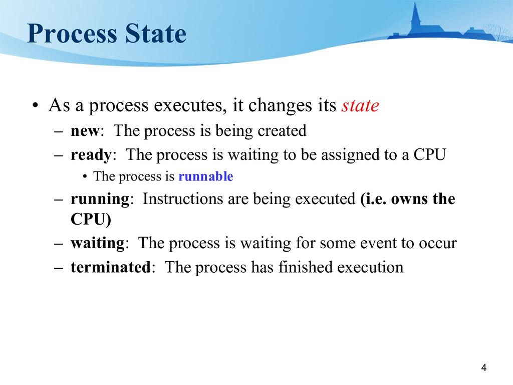
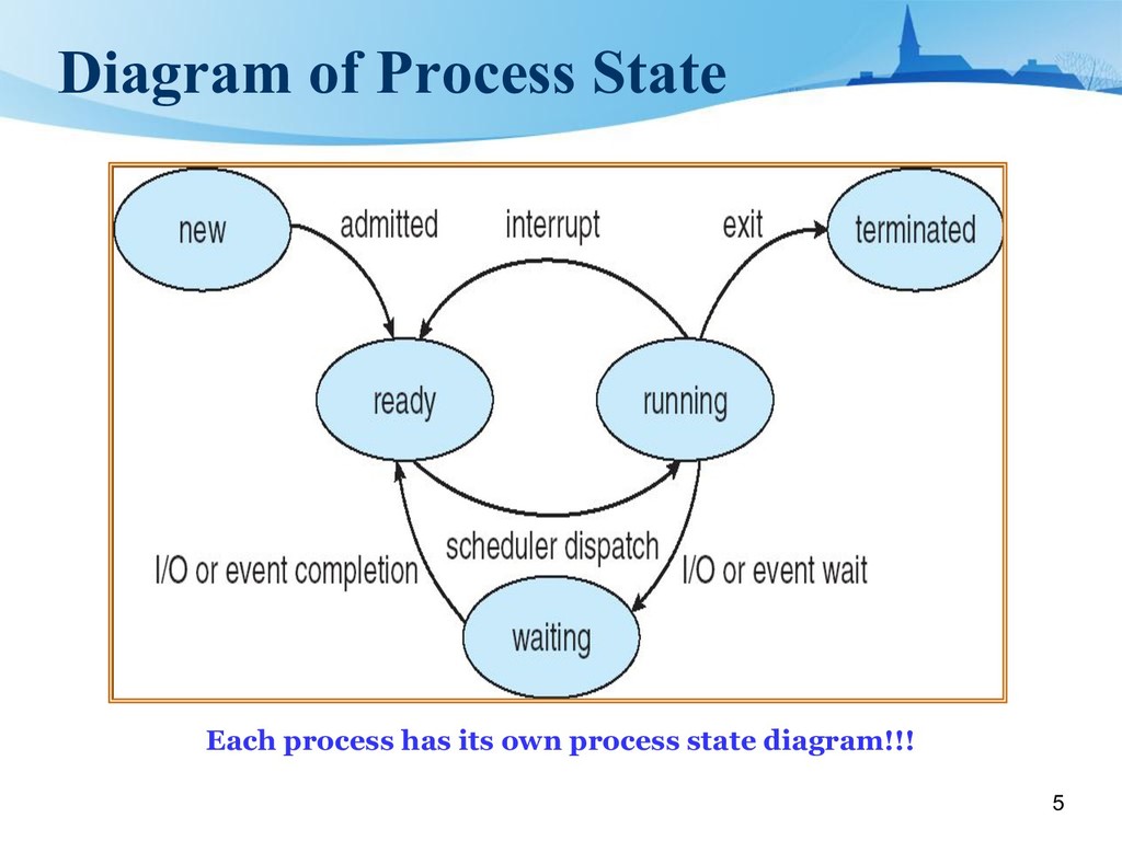
its state – new: The process is being created – ready: The process is waiting to be assigned to a CPU • The process is runnable – running: Instructions are being executed (i.e. owns the CPU) – waiting: The process is waiting for some event to occur – terminated: The process has finished execution
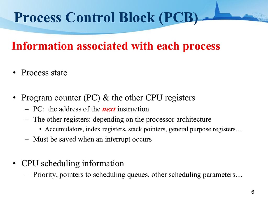
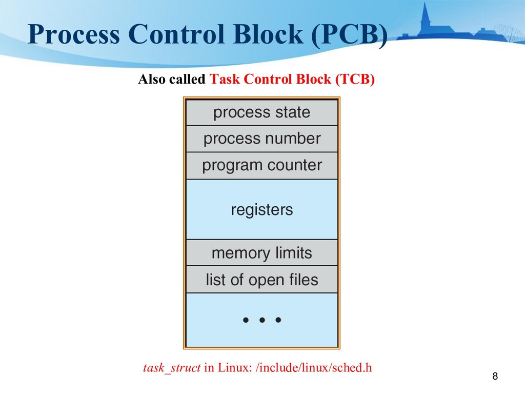
• Process state • Program counter (PC) & the other CPU registers – PC: the address of the next instruction – The other registers: depending on the processor architecture • Accumulators, index registers, stack pointers, general purpose registers… – Must be saved when an interrupt occurs • CPU scheduling information – Priority, pointers to scheduling queues, other scheduling parameters…
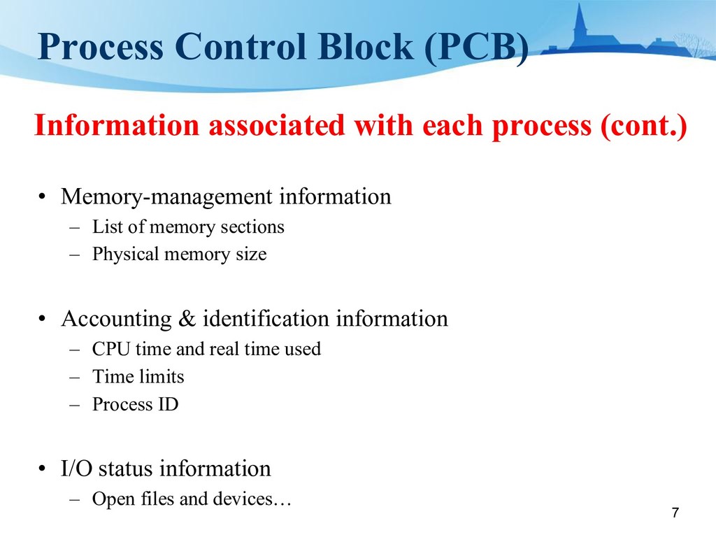
(cont.) • Memory-management information – List of memory sections – Physical memory size • Accounting & identification information – CPU time and real time used – Time limits – Process ID • I/O status information – Open files and devices…
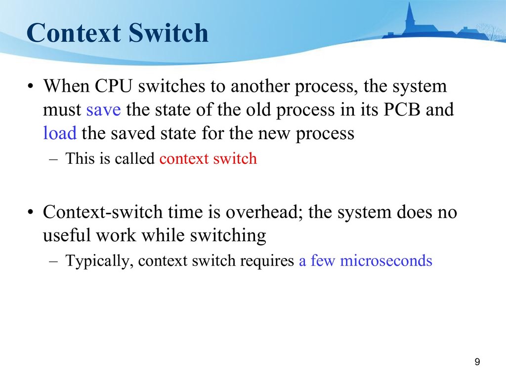
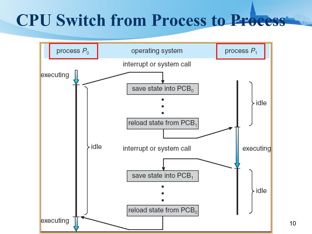
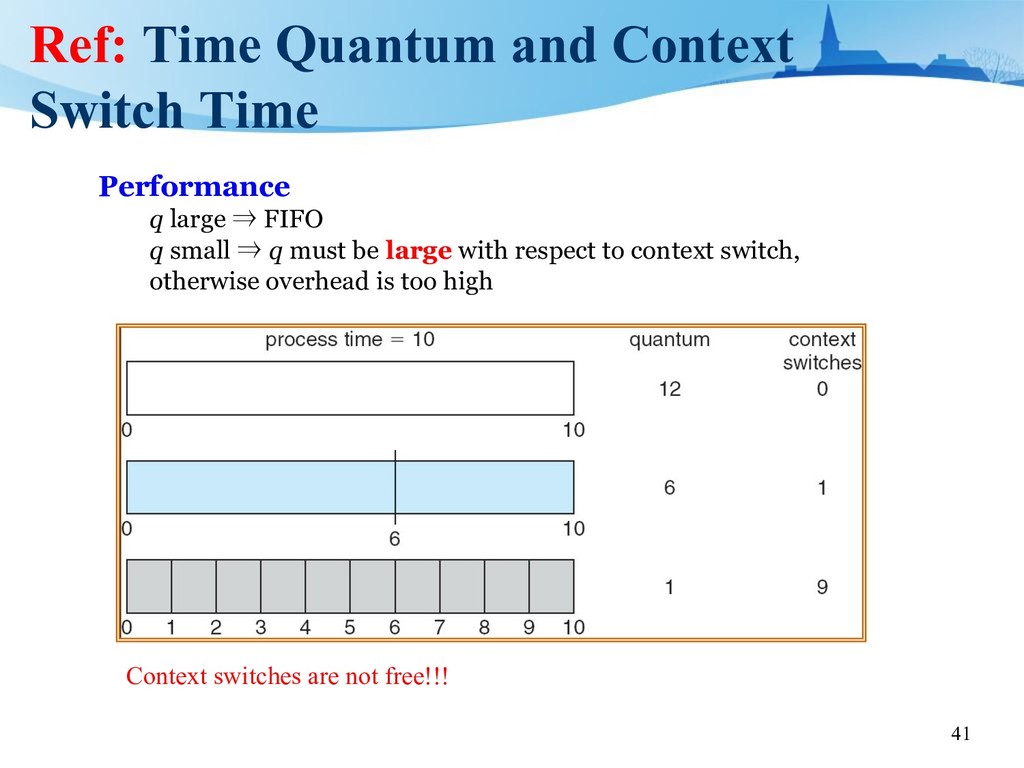
the system must save the state of the old process in its PCB and load the saved state for the new process – This is called context switch • Context-switch time is overhead; the system does no useful work while switching – Typically, context switch requires a few microseconds
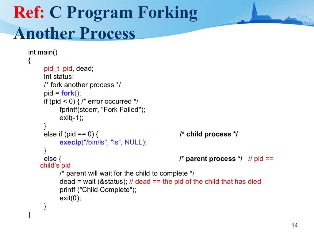
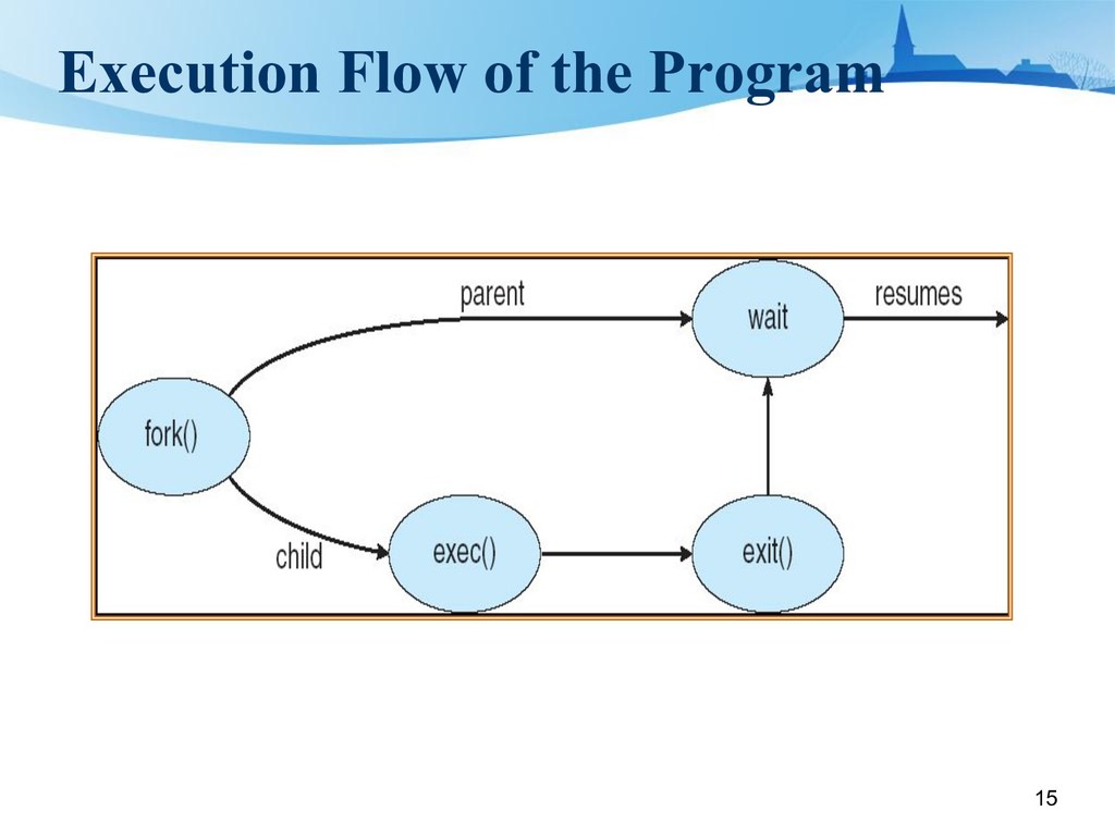
pid_t pid, dead; int status; /* fork another process */ pid = fork(); if (pid < 0) { /* error occurred */ fprintf(stderr, "Fork Failed"); exit(-1); } else if (pid == 0) { /* child process */ execlp("/bin/ls", "ls", NULL); } else { /* parent process */ // pid == child’s pid /* parent will wait for the child to complete */ dead = wait (&status); // dead == the pid of the child that has died printf ("Child Complete"); exit(0); } }
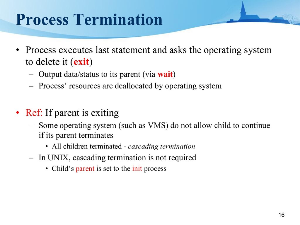
the operating system to delete it (exit) – Output data/status to its parent (via wait) – Process’ resources are deallocated by operating system • Ref: If parent is exiting – Some operating system (such as VMS) do not allow child to continue if its parent terminates • All children terminated - cascading termination – In UNIX, cascading termination is not required • Child’s parent is set to the init process
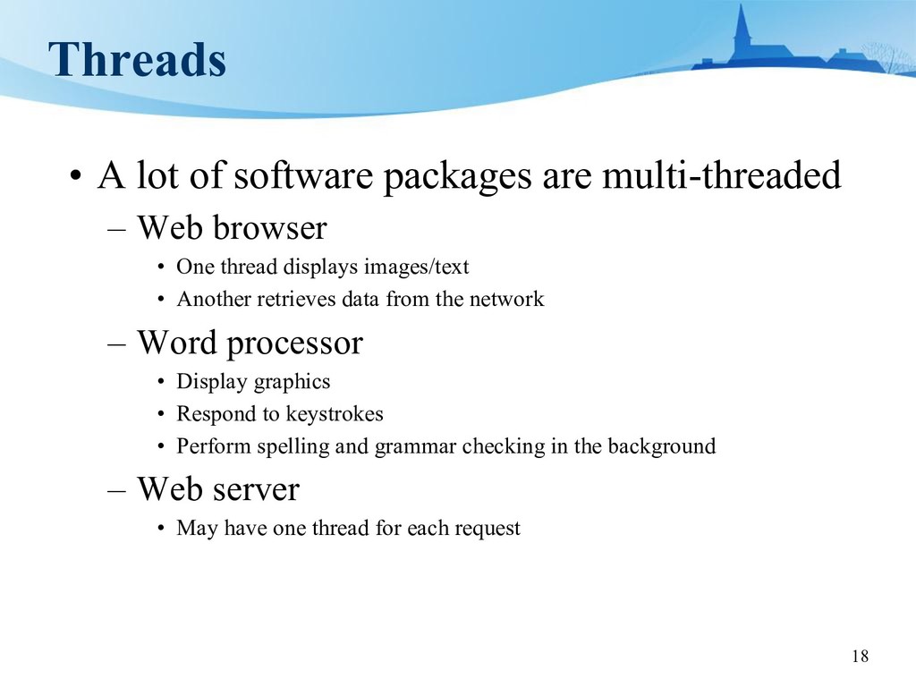
– Web browser • One thread displays images/text • Another retrieves data from the network – Word processor • Display graphics • Respond to keystrokes • Perform spelling and grammar checking in the background – Web server • May have one thread for each request
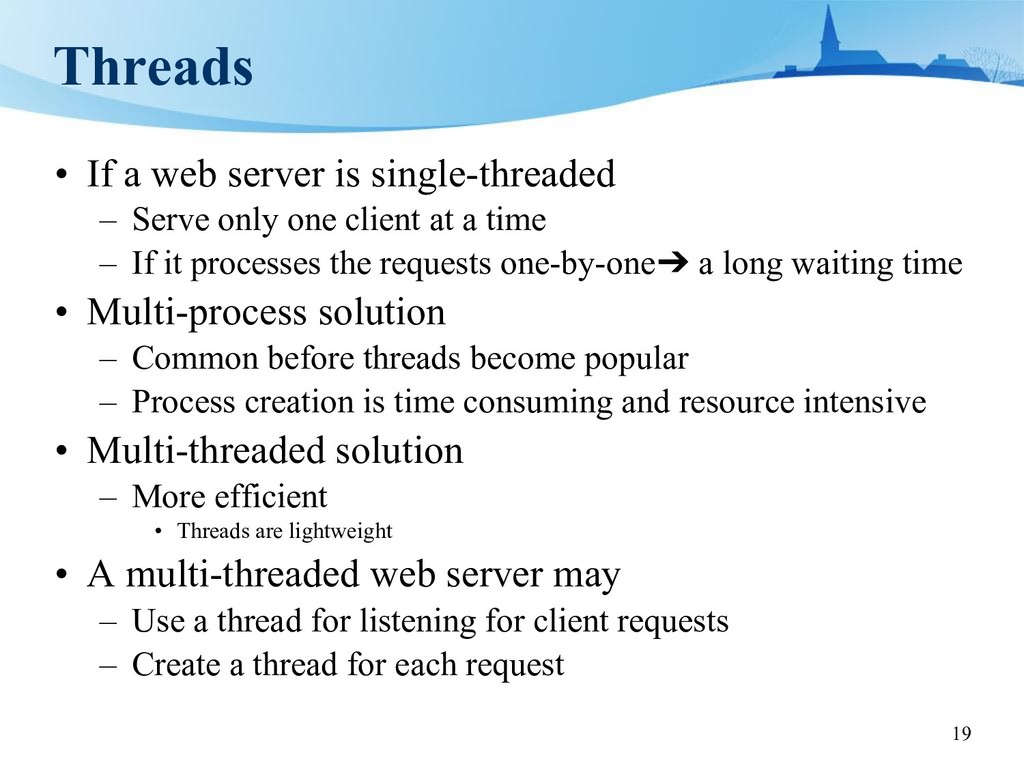
Serve only one client at a time – If it processes the requests one-by-one➔ a long waiting time • Multi-process solution – Common before threads become popular – Process creation is time consuming and resource intensive • Multi-threaded solution – More efficient • Threads are lightweight • A multi-threaded web server may – Use a thread for listening for client requests – Create a thread for each request
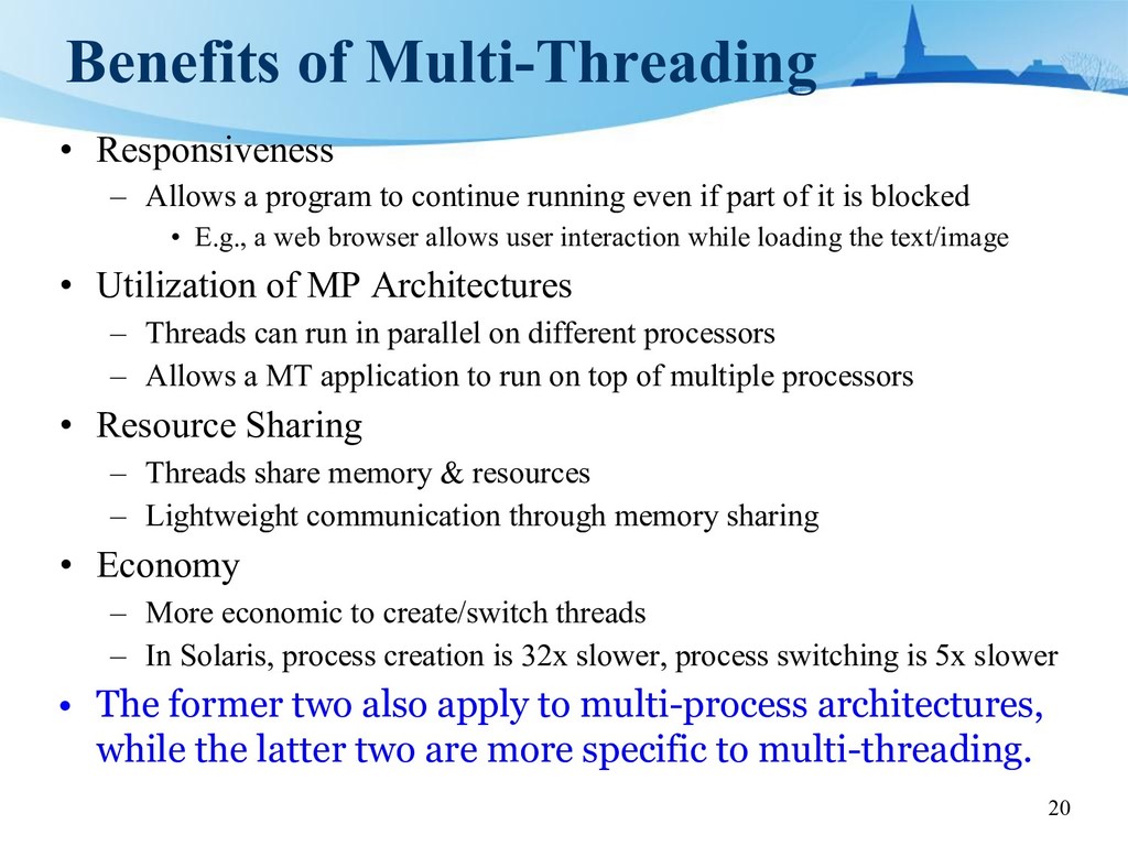
to continue running even if part of it is blocked • E.g., a web browser allows user interaction while loading the text/image • Utilization of MP Architectures – Threads can run in parallel on different processors – Allows a MT application to run on top of multiple processors • Resource Sharing – Threads share memory & resources – Lightweight communication through memory sharing • Economy – More economic to create/switch threads – In Solaris, process creation is 32x slower, process switching is 5x slower • The former two also apply to multi-process architectures, while the latter two are more specific to multi-threading.
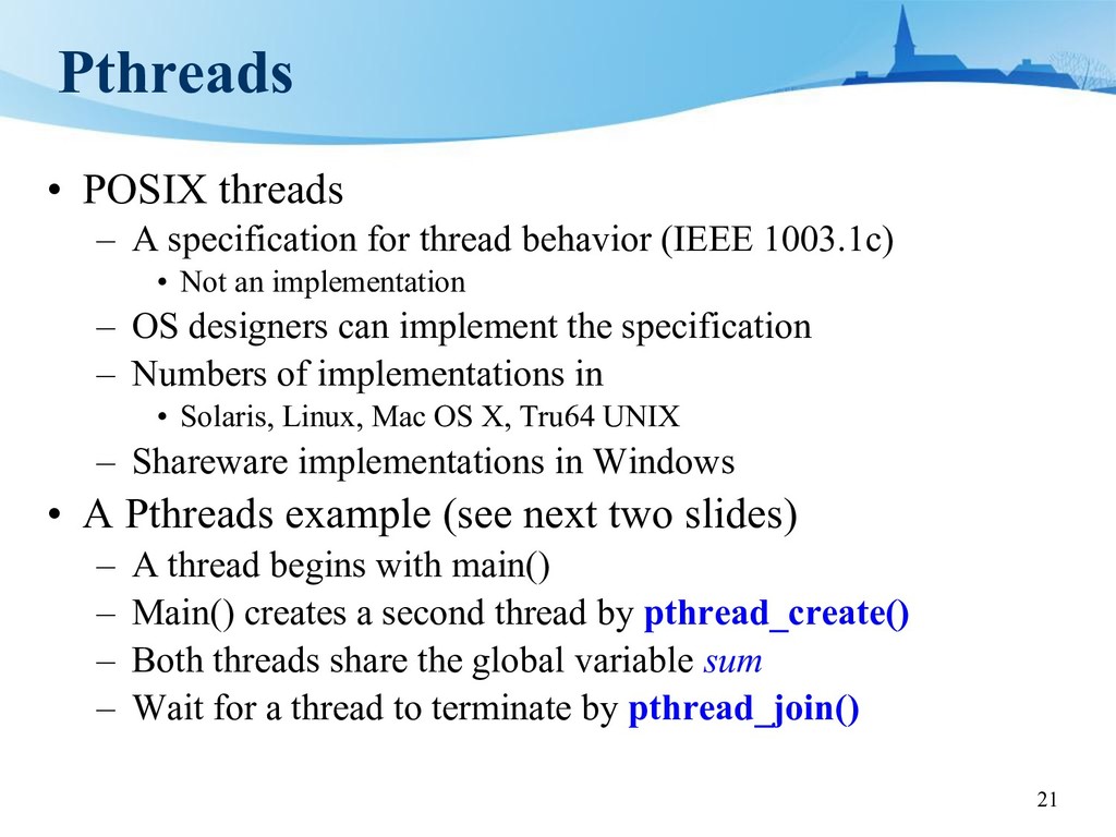
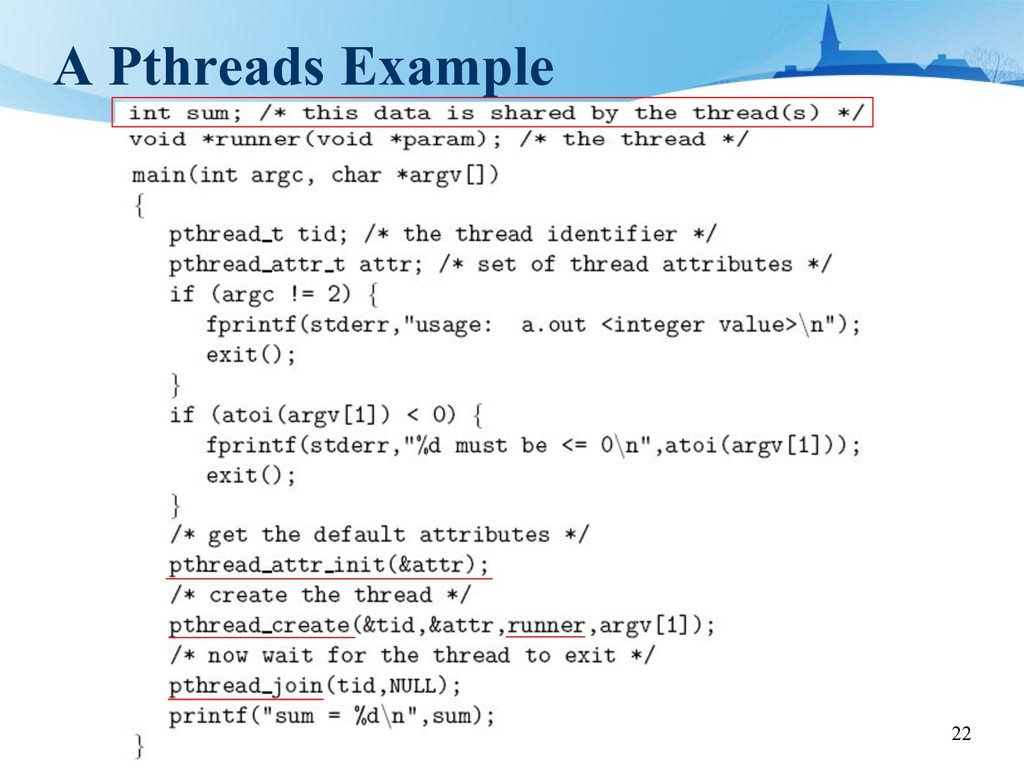
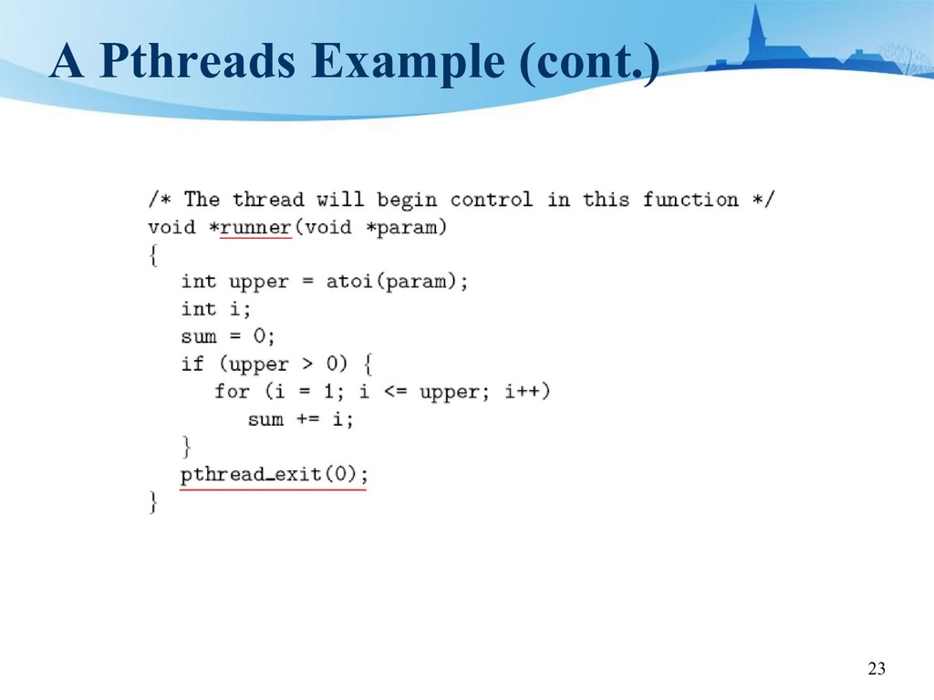
behavior (IEEE 1003.1c) • Not an implementation – OS designers can implement the specification – Numbers of implementations in • Solaris, Linux, Mac OS X, Tru64 UNIX – Shareware implementations in Windows • A Pthreads example (see next two slides) – A thread begins with main() – Main() creates a second thread by pthread_create() – Both threads share the global variable sum – Wait for a thread to terminate by pthread_join()
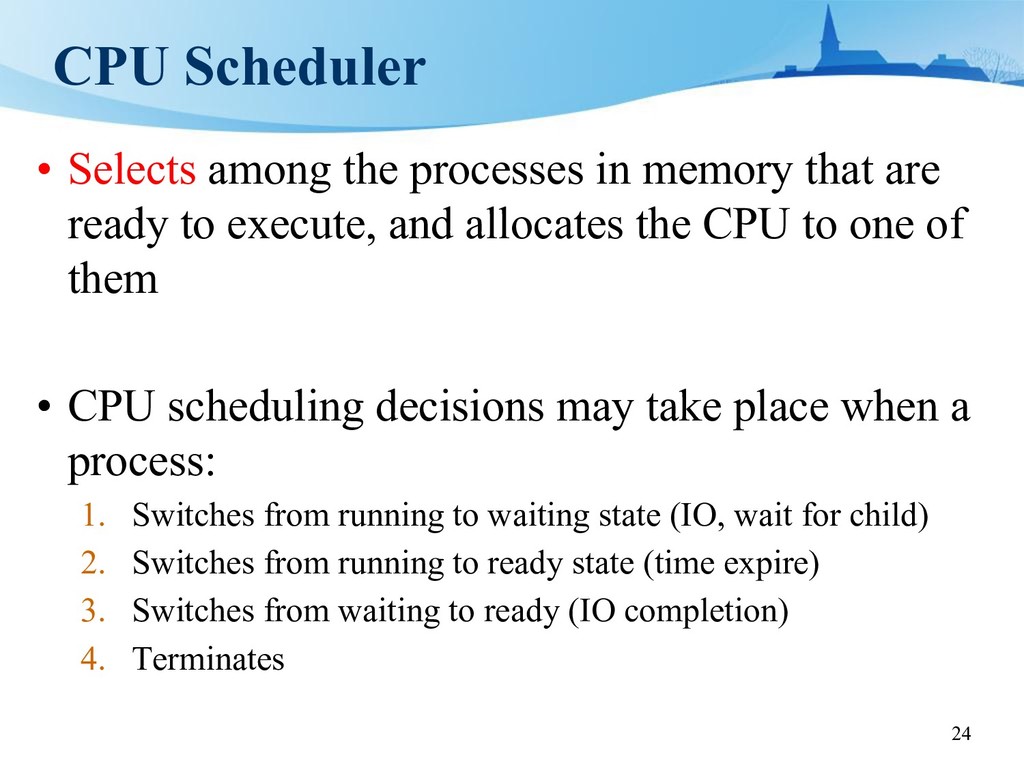
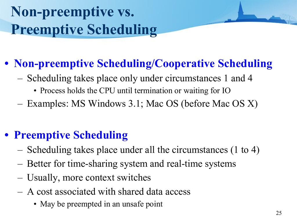
that are ready to execute, and allocates the CPU to one of them • CPU scheduling decisions may take place when a process: 1. Switches from running to waiting state (IO, wait for child) 2. Switches from running to ready state (time expire) 3. Switches from waiting to ready (IO completion) 4. Terminates
Scheduling takes place only under circumstances 1 and 4 • Process holds the CPU until termination or waiting for IO – Examples: MS Windows 3.1; Mac OS (before Mac OS X) • Preemptive Scheduling – Scheduling takes place under all the circumstances (1 to 4) – Better for time-sharing system and real-time systems – Usually, more context switches – A cost associated with shared data access • May be preempted in an unsafe point
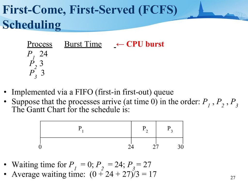
burst P 1 24 P 2 3 P 3 3 • Implemented via a FIFO (first-in first-out) queue • Suppose that the processes arrive (at time 0) in the order: P 1 , P 2 , P 3 The Gantt Chart for the schedule is: • Waiting time for P 1 = 0; P 2 = 24; P 3 = 27 • Average waiting time: (0 + 24 + 27)/3 = 17 P 1 P 2 P 3 24 27 30 0
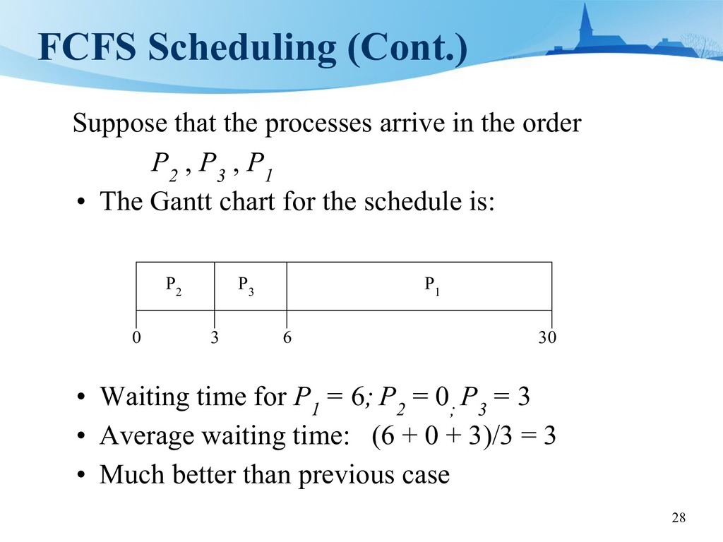
the order P 2 , P 3 , P 1 • The Gantt chart for the schedule is: • Waiting time for P 1 = 6; P 2 = 0 ; P 3 = 3 • Average waiting time: (6 + 0 + 3)/3 = 3 • Much better than previous case P 1 P 3 P 2 6 3 30 0
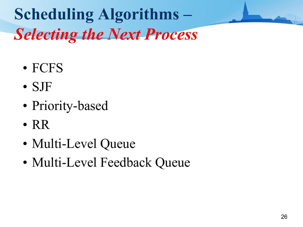
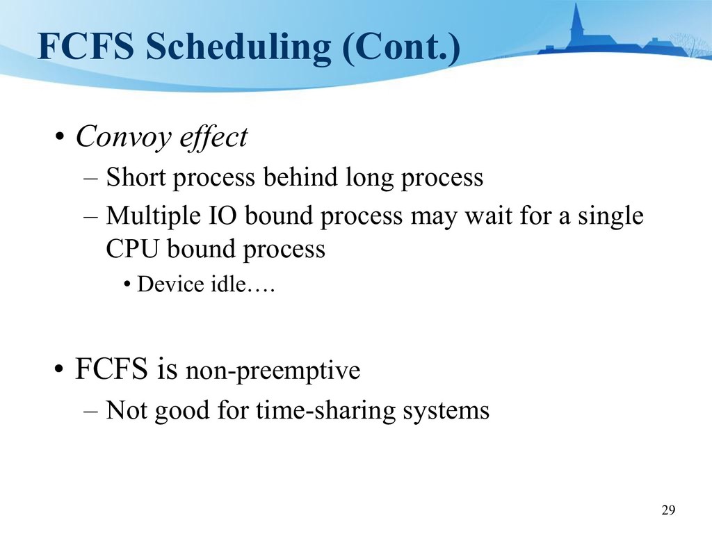
behind long process – Multiple IO bound process may wait for a single CPU bound process • Device idle…. • FCFS is non-preemptive – Not good for time-sharing systems
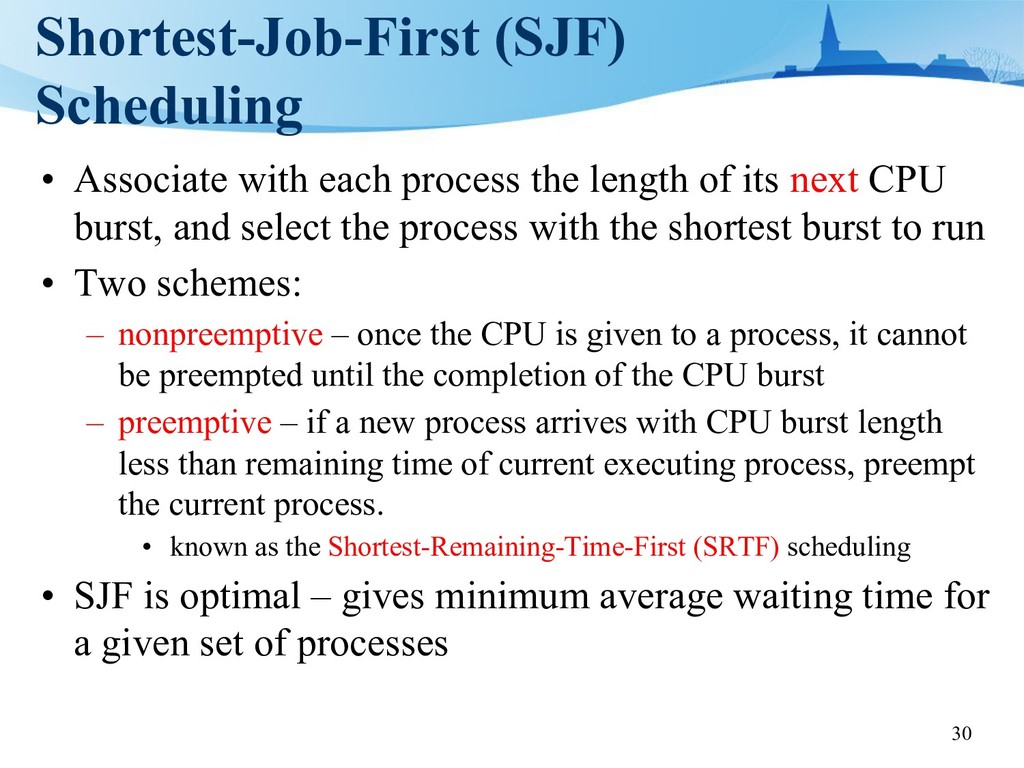
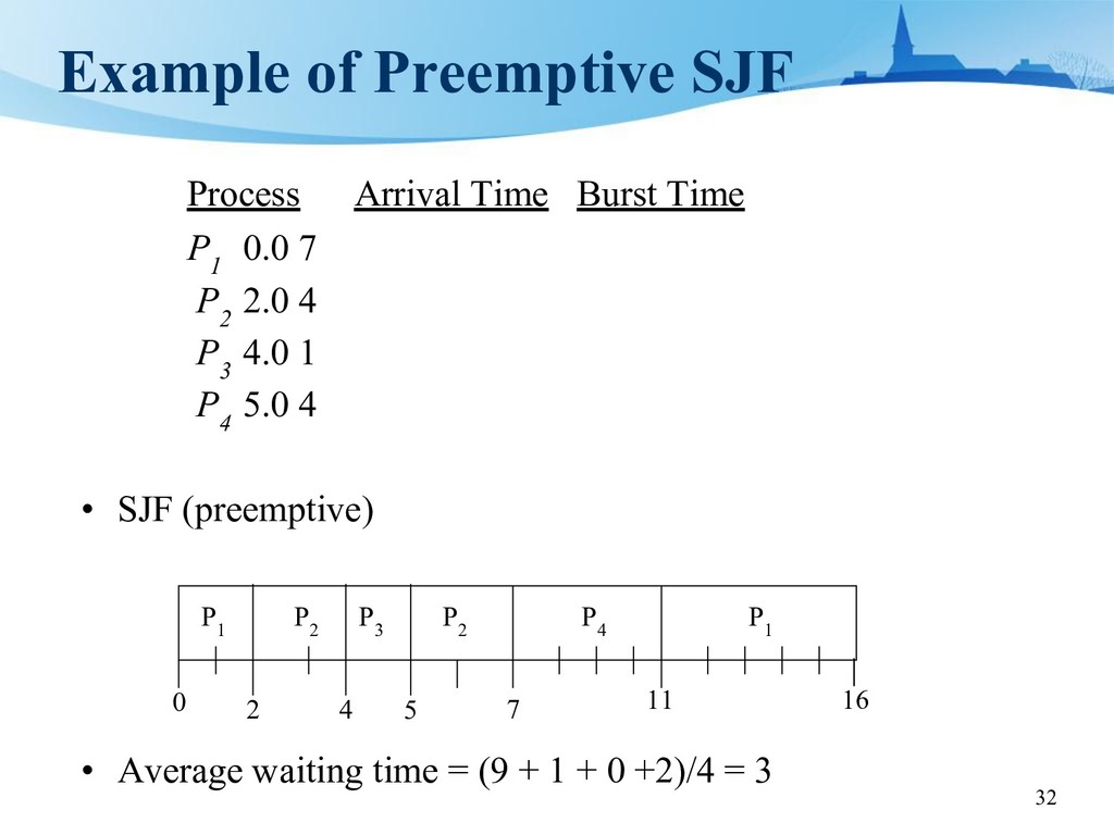
length of its next CPU burst, and select the process with the shortest burst to run • Two schemes: – nonpreemptive – once the CPU is given to a process, it cannot be preempted until the completion of the CPU burst – preemptive – if a new process arrives with CPU burst length less than remaining time of current executing process, preempt the current process. • known as the Shortest-Remaining-Time-First (SRTF) scheduling • SJF is optimal – gives minimum average waiting time for a given set of processes
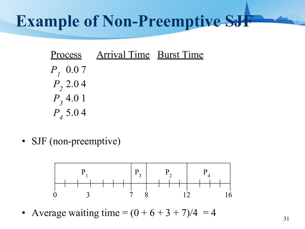
P 2 2.0 4 P 3 4.0 1 P 4 5.0 4 • SJF (non-preemptive) • Average waiting time = (0 + 6 + 3 + 7)/4 = 4 Example of Non-Preemptive SJF P 1 P 3 P 2 7 3 16 0 P 4 8 12
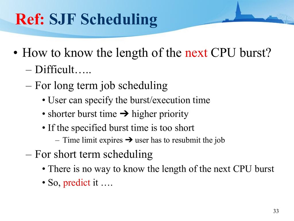
of the next CPU burst? – Difficult….. – For long term job scheduling • User can specify the burst/execution time • shorter burst time ➔ higher priority • If the specified burst time is too short – Time limit expires ➔ user has to resubmit the job – For short term scheduling • There is no way to know the length of the next CPU burst • So, predict it ….
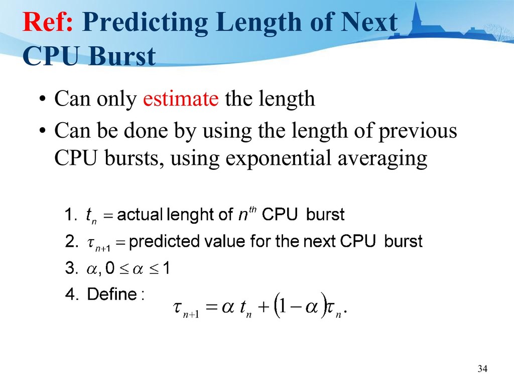
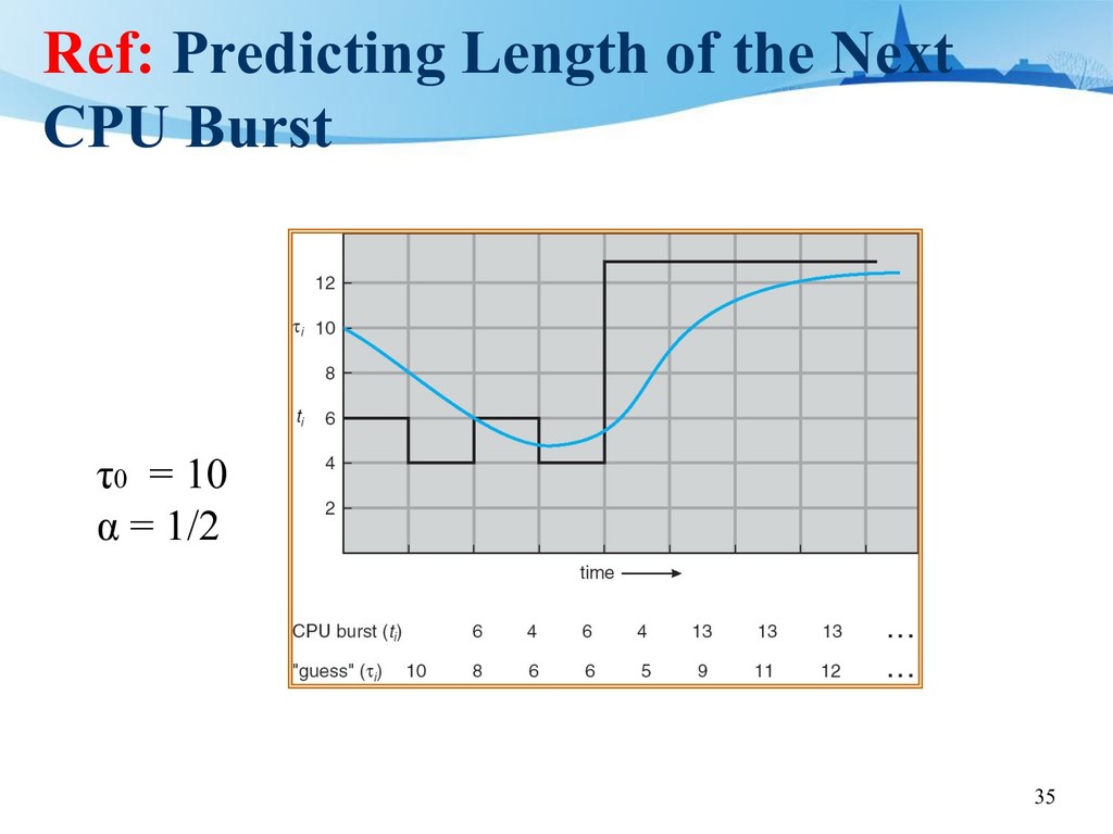
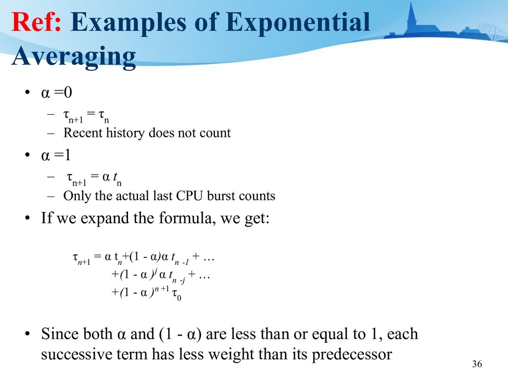
τ n+1 = τ n – Recent history does not count • α =1 – τ n+1 = α t n – Only the actual last CPU burst counts • If we expand the formula, we get: τ n+1 = α t n +(1 - α)α t n -1 + … +(1 - α )j α t n -j + … +(1 - α )n +1 τ 0 • Since both α and (1 - α) are less than or equal to 1, each successive term has less weight than its predecessor
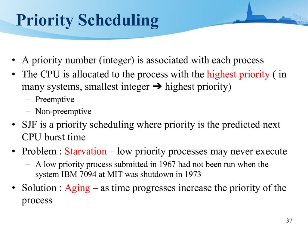
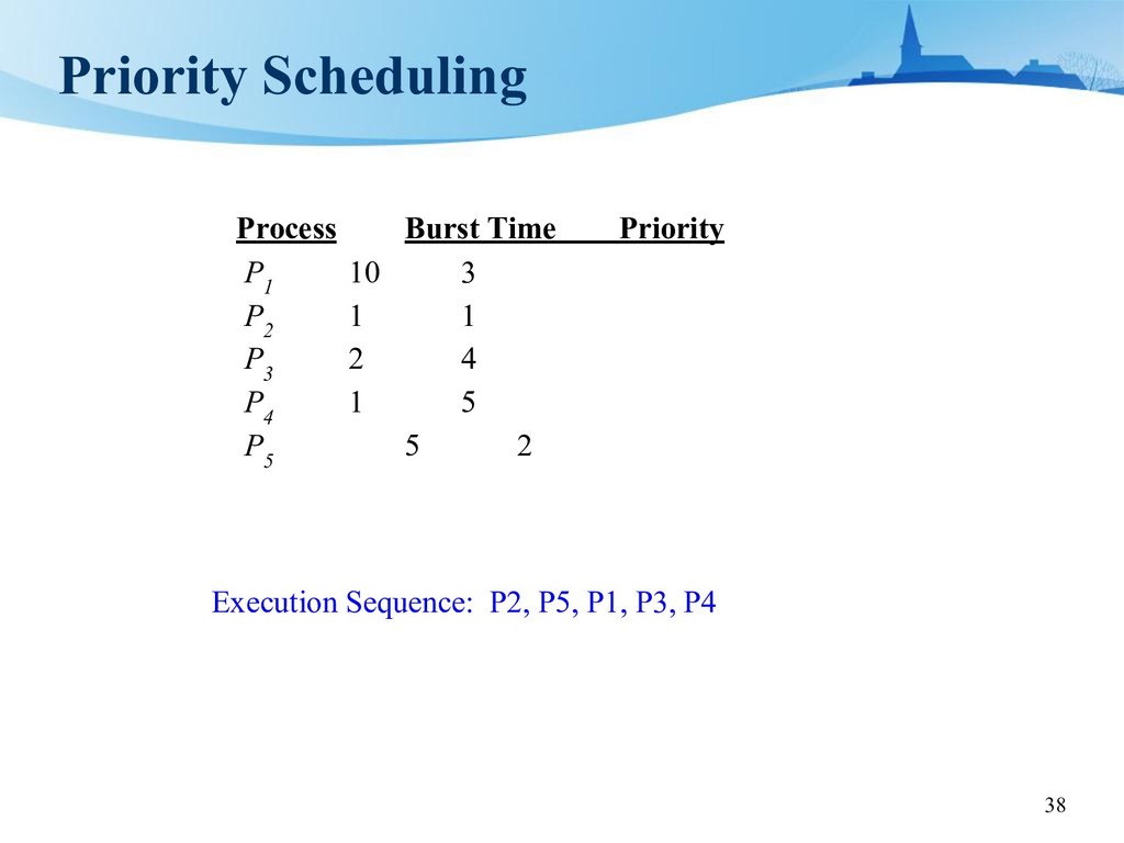
with each process • The CPU is allocated to the process with the highest priority ( in many systems, smallest integer ➔ highest priority) – Preemptive – Non-preemptive • SJF is a priority scheduling where priority is the predicted next CPU burst time • Problem : Starvation – low priority processes may never execute – A low priority process submitted in 1967 had not been run when the system IBM 7094 at MIT was shutdown in 1973 • Solution : Aging – as time progresses increase the priority of the process
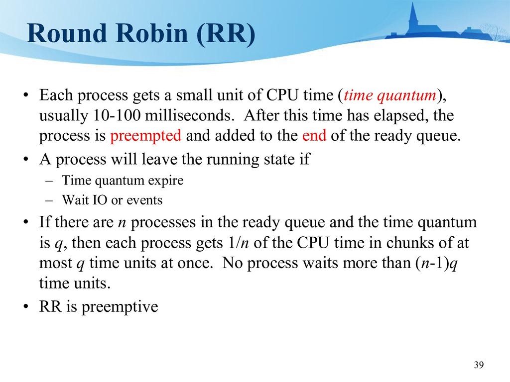
unit of CPU time (time quantum), usually 10-100 milliseconds. After this time has elapsed, the process is preempted and added to the end of the ready queue. • A process will leave the running state if – Time quantum expire – Wait IO or events • If there are n processes in the ready queue and the time quantum is q, then each process gets 1/n of the CPU time in chunks of at most q time units at once. No process waits more than (n-1)q time units. • RR is preemptive
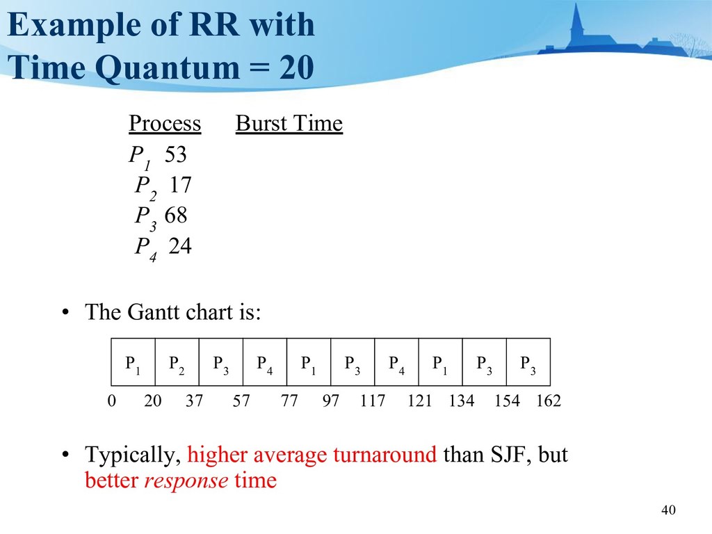
Burst Time P 1 53 P 2 17 P 3 68 P 4 24 • The Gantt chart is: • Typically, higher average turnaround than SJF, but better response time P 1 P 2 P 3 P 4 P 1 P 3 P 4 P 1 P 3 P 3 0 20 37 57 77 97 117 121 134 154 162
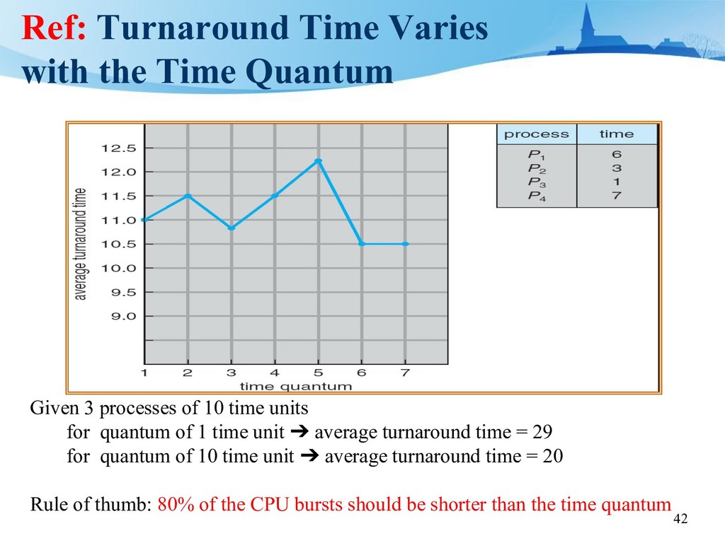
3 processes of 10 time units for quantum of 1 time unit ➔ average turnaround time = 29 for quantum of 10 time unit ➔ average turnaround time = 20 Rule of thumb: 80% of the CPU bursts should be shorter than the time quantum
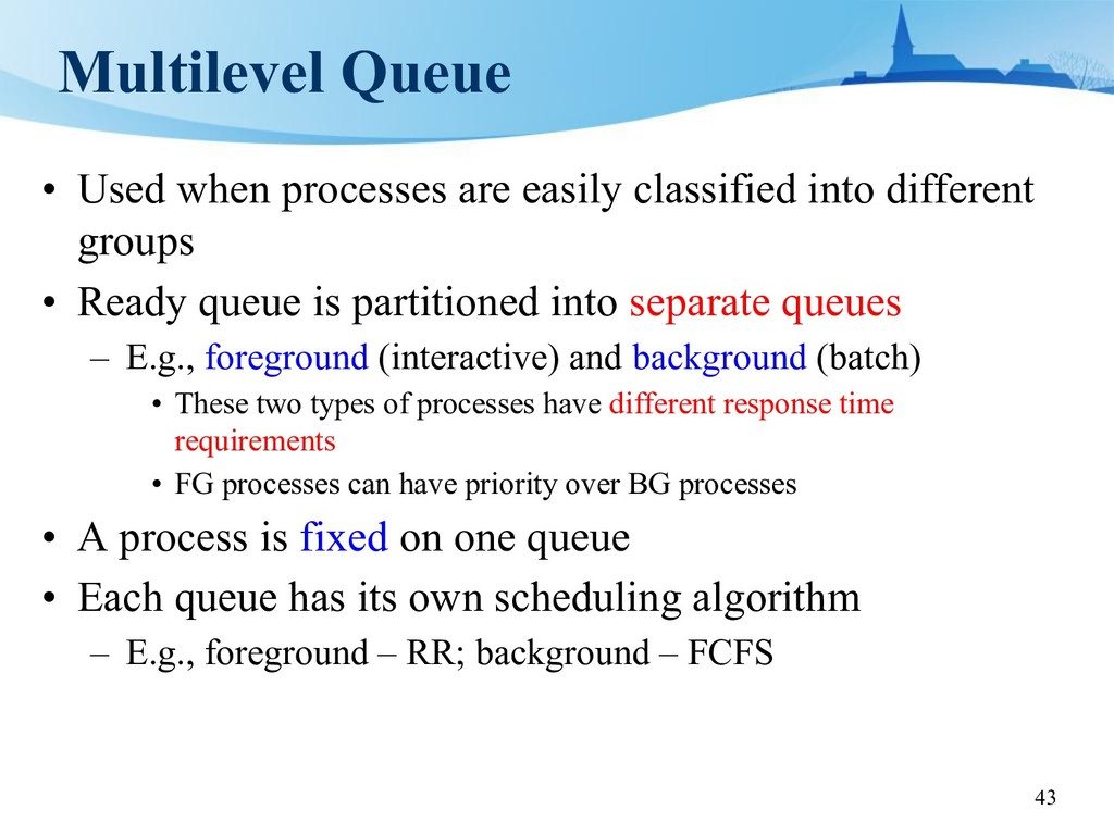
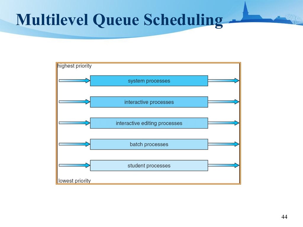
into different groups • Ready queue is partitioned into separate queues – E.g., foreground (interactive) and background (batch) • These two types of processes have different response time requirements • FG processes can have priority over BG processes • A process is fixed on one queue • Each queue has its own scheduling algorithm – E.g., foreground – RR; background – FCFS
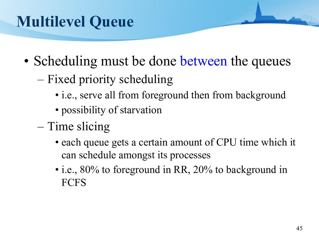
queues – Fixed priority scheduling • i.e., serve all from foreground then from background • possibility of starvation – Time slicing • each queue gets a certain amount of CPU time which it can schedule amongst its processes • i.e., 80% to foreground in RR, 20% to background in FCFS
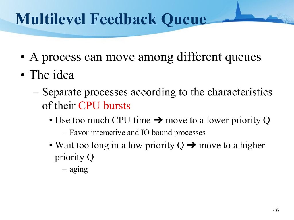
different queues • The idea – Separate processes according to the characteristics of their CPU bursts • Use too much CPU time ➔ move to a lower priority Q – Favor interactive and IO bound processes • Wait too long in a low priority Q ➔ move to a higher priority Q – aging
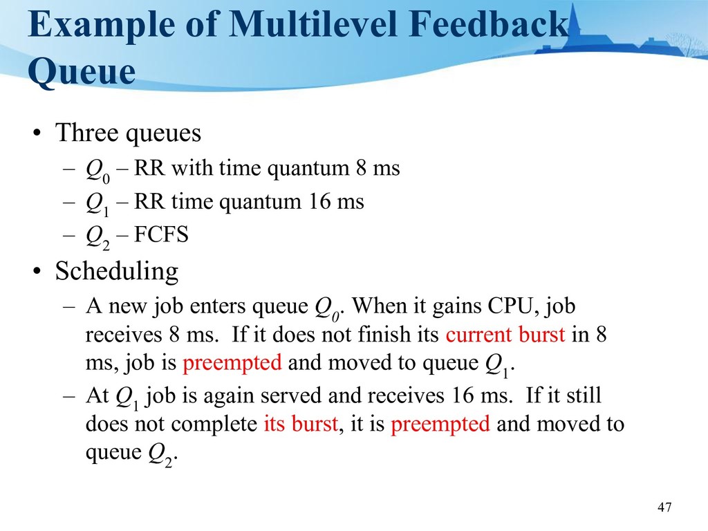
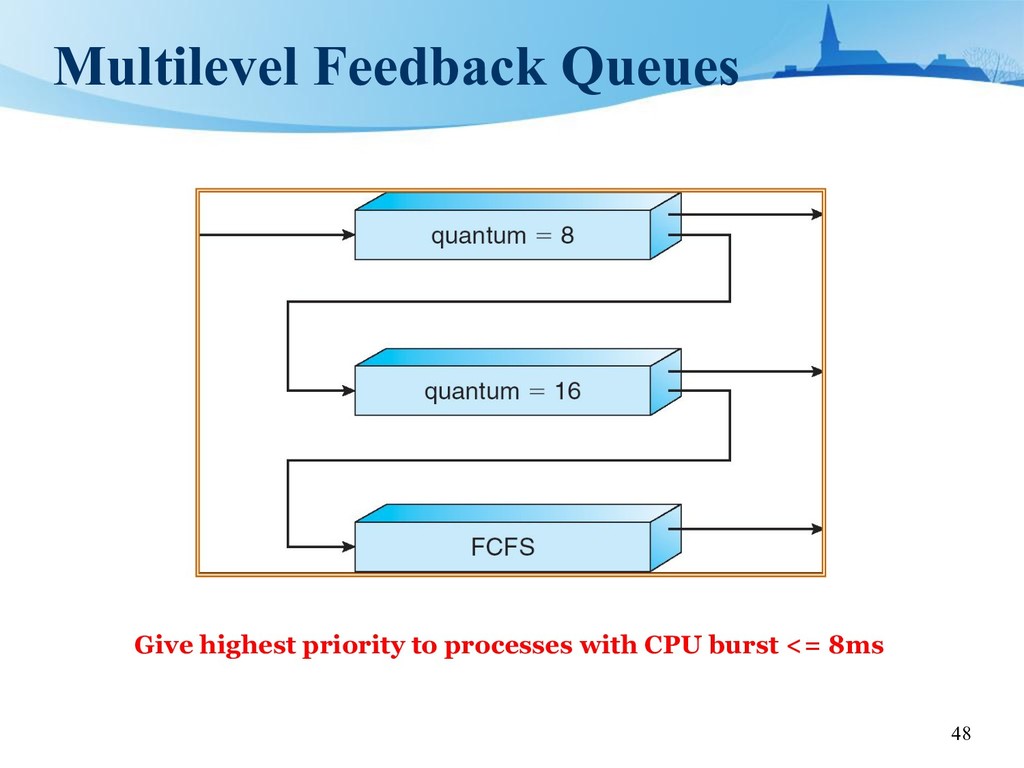
Q 0 – RR with time quantum 8 ms – Q 1 – RR time quantum 16 ms – Q 2 – FCFS • Scheduling – A new job enters queue Q 0 . When it gains CPU, job receives 8 ms. If it does not finish its current burst in 8 ms, job is preempted and moved to queue Q 1 . – At Q 1 job is again served and receives 16 ms. If it still does not complete its burst, it is preempted and moved to queue Q 2 .
following parameters: – number of queues – scheduling algorithms for each queue – method used to determine when to promote a process – method used to determine when to demote a process – method used to determine which queue a process will enter when that process needs service • It is the most generic algorithm – Can be configured to match a specific system • It is the most complex algorithm – You have to select a proper value for each parameter

 SiteGround - Reliable hosting with speed, security, and support you can count on.


 xvillage
 koic
koic
 kanfab1
 oga5
oga5
 panda728
 lynnswap
 ktcryomm
 koher
koher
 y0hgi
y0hgi
 tsutsui
 marcoroth
 sts11142
 willnet
 kneath
 cassininazir
 rasagy
 ammeep
 aleyda
 honzajavorek
 reverentgeek
 jcasabona
 bermonpainter
 davetheseo
 eileencodes