On-line and Dynamic Estimation of Rician Fading Channels in GSM-R Networks

WCSP '2012

Transcript

1. On-line and Dynamic Estimation of Rician Fading Channels in GSM-R Networks Yongsen Ma Pengyuan Du Xiaofeng Mao Chengnian Long International Conference on Wireless Communications and Signal Processing October 16, 2012 Yongsen Ma (SJTU) On-line Estimation of Rician Fading Channels WCSP ’12 - WCS 1 / 31
2. Outline 1 Introduction Background Propagation Models Measurement Procedures 2 On-line Estimation Measurement Framework Length of Statistical Intervals Number of Averaging Samples 3 Performance Evaluation Implementation Experiment Evaluation Yongsen Ma (SJTU) On-line Estimation of Rician Fading Channels WCSP ’12 - WCS 2 / 31
3. Outline 1 Introduction Background Propagation Models Measurement Procedures 2 On-line Estimation Measurement Framework Length of Statistical Intervals Number of Averaging Samples 3 Performance Evaluation Implementation Experiment Evaluation Yongsen Ma (SJTU) On-line Estimation of Rician Fading Channels WCSP ’12 - WCS 3 / 31
4. Background GSM-R for high-speed railway The high-speed railway is critical for transporting commodities and passengers, and it has experienced rapid development recently. The primary consideration of high-speed railway is safety, which increasingly relies on the information and communication system. So it requires realtime measurement to ensure the reliability and stability of GSM-R networks and the high-speed railway system.1 1 G. Baldini, etc. An early warning system for detecting GSM-R wireless interference in the high-speed railway infrastructure. International Journal of Critical Infrastructure Protection, 2010. Yongsen Ma (SJTU) On-line Estimation of Rician Fading Channels WCSP ’12 - WCS 4 / 31
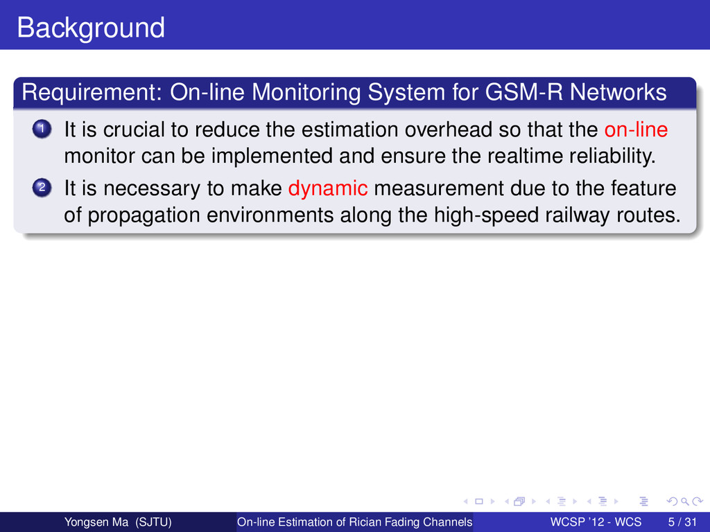
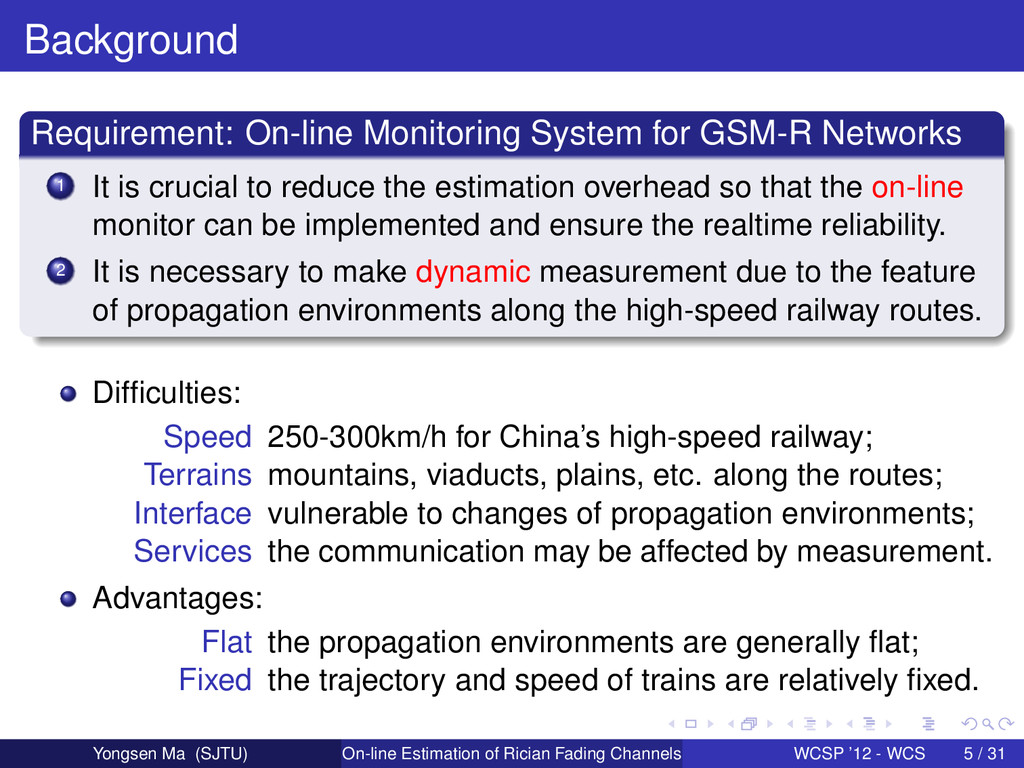
5. Background Requirement: On-line Monitoring System for GSM-R Networks 1 It is crucial to reduce the estimation overhead so that the on-line monitor can be implemented and ensure the realtime reliability. 2 It is necessary to make dynamic measurement due to the feature of propagation environments along the high-speed railway routes. Yongsen Ma (SJTU) On-line Estimation of Rician Fading Channels WCSP ’12 - WCS 5 / 31
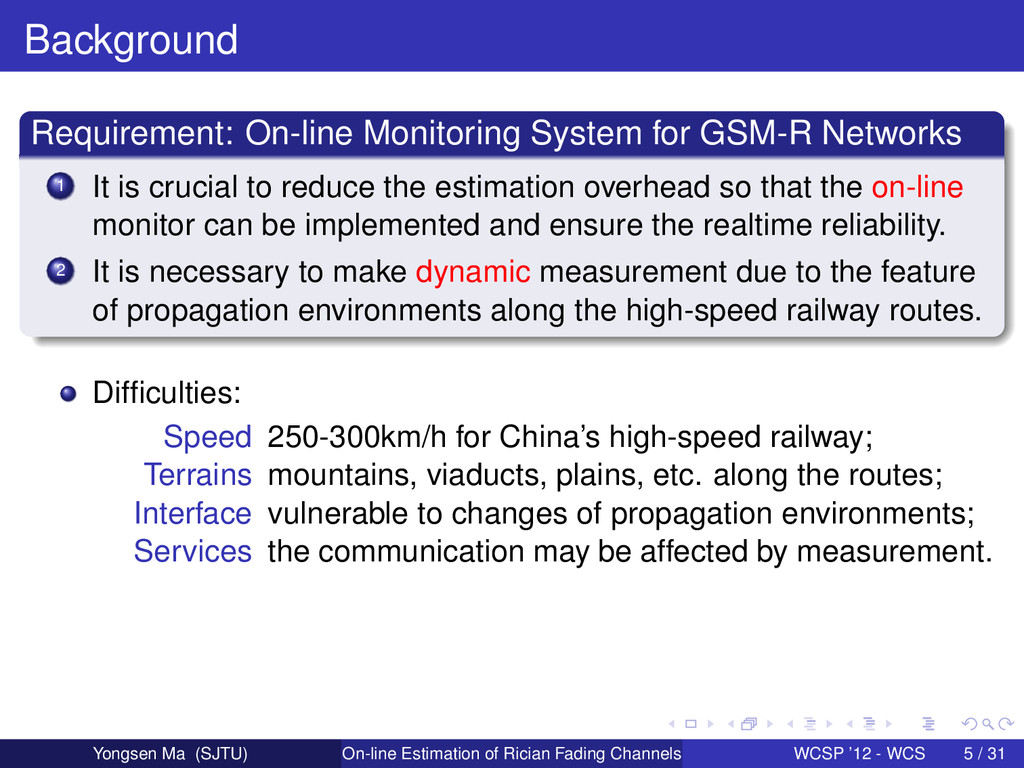
6. Background Requirement: On-line Monitoring System for GSM-R Networks 1 It is crucial to reduce the estimation overhead so that the on-line monitor can be implemented and ensure the realtime reliability. 2 It is necessary to make dynamic measurement due to the feature of propagation environments along the high-speed railway routes. Difficulties: Speed 250-300km/h for China’s high-speed railway; Terrains mountains, viaducts, plains, etc. along the routes; Interface vulnerable to changes of propagation environments; Services the communication may be affected by measurement. Yongsen Ma (SJTU) On-line Estimation of Rician Fading Channels WCSP ’12 - WCS 5 / 31
7. Background Requirement: On-line Monitoring System for GSM-R Networks 1 It is crucial to reduce the estimation overhead so that the on-line monitor can be implemented and ensure the realtime reliability. 2 It is necessary to make dynamic measurement due to the feature of propagation environments along the high-speed railway routes. Difficulties: Speed 250-300km/h for China’s high-speed railway; Terrains mountains, viaducts, plains, etc. along the routes; Interface vulnerable to changes of propagation environments; Services the communication may be affected by measurement. Advantages: Flat the propagation environments are generally flat; Fixed the trajectory and speed of trains are relatively fixed. Yongsen Ma (SJTU) On-line Estimation of Rician Fading Channels WCSP ’12 - WCS 5 / 31
8. Background Lee’s method proposed a standard process of local mean power estimation, which is determined in Rayleigh fading channels.2 The Generalized Lee method does not need a priori knowing the distribution function, but the optimum length of averaging interval is calculated by all the routes of the database with high overhead.3 2 W.C.Y. Lee. Estimate of local average power of a mobile radio signal.IEEE Transactions on Vehicular Technology, 1985. 3 D. de la Vega, etc. Generalization of the Lee method for the analysis of the signal variability. IEEE Transactions on Vehicular Technology, 2009. Yongsen Ma (SJTU) On-line Estimation of Rician Fading Channels WCSP ’12 - WCS 6 / 31
9. Outline 1 Introduction Background Propagation Models Measurement Procedures 2 On-line Estimation Measurement Framework Length of Statistical Intervals Number of Averaging Samples 3 Performance Evaluation Implementation Experiment Evaluation Yongsen Ma (SJTU) On-line Estimation of Rician Fading Channels WCSP ’12 - WCS 7 / 31
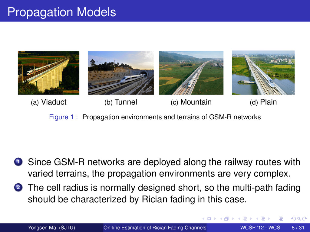
10. Propagation Models (a) Viaduct (b) Tunnel (c) Mountain (d) Plain Figure 1 : Propagation environments and terrains of GSM-R networks 1 Since GSM-R networks are deployed along the railway routes with varied terrains, the propagation environments are very complex. 2 The cell radius is normally designed short, so the multi-path fading should be characterized by Rician fading in this case. Yongsen Ma (SJTU) On-line Estimation of Rician Fading Channels WCSP ’12 - WCS 8 / 31
11. Propagation Models p2 r (x) = s(x)h(x) (1) 1 Shadowing fading: s(x) ∼ N m(x), σ2 s (2) 2 Multi-path fading: h(x) = 1 √ 1 + K lim M→∞ 1 √ M M m=1 amej(2π λ cos(θmx)+φm ) NLOS Components + K 1 + K ej( 2π λ cos(θ0x+φ0)) LOS Component (3) Yongsen Ma (SJTU) On-line Estimation of Rician Fading Channels WCSP ’12 - WCS 9 / 31
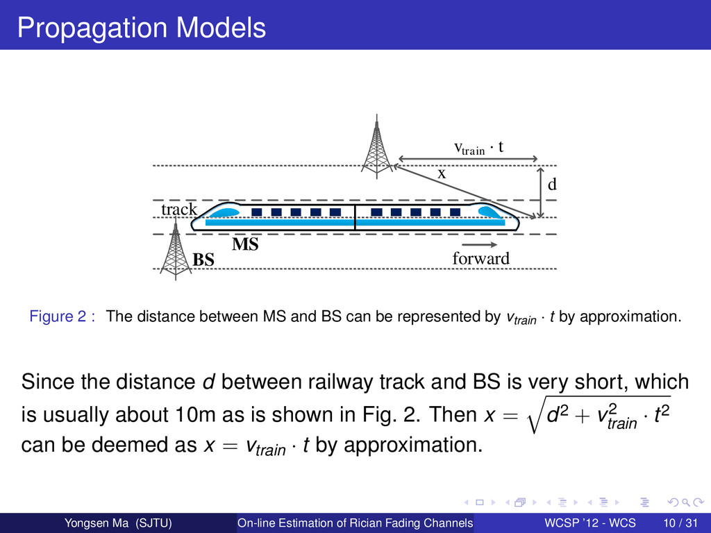
12. Propagation Models d x vtrain · t forward track BS MS Figure 2 : The distance between MS and BS can be represented by vtrain · t by approximation. Since the distance d between railway track and BS is very short, which is usually about 10m as is shown in Fig. 2. Then x = d2 + v2 train · t2 can be deemed as x = vtrain · t by approximation. Yongsen Ma (SJTU) On-line Estimation of Rician Fading Channels WCSP ’12 - WCS 10 / 31
13. Outline 1 Introduction Background Propagation Models Measurement Procedures 2 On-line Estimation Measurement Framework Length of Statistical Intervals Number of Averaging Samples 3 Performance Evaluation Implementation Experiment Evaluation Yongsen Ma (SJTU) On-line Estimation of Rician Fading Channels WCSP ’12 - WCS 11 / 31
14. Measurement Procedures Local Power Estimation Received Signal AMP Propagation Prediction Model Correction ) (x P r ) (x S ) (x M 2 1 , K K Figure 3 : Basic Procedures of Radio Propagation Measurement The procedures of propagation measurement in GSM-R networks is typically composed of the local mean power estimation, propagation prediction and model correction, as is demonstrated in Fig. 3. Yongsen Ma (SJTU) On-line Estimation of Rician Fading Channels WCSP ’12 - WCS 12 / 31
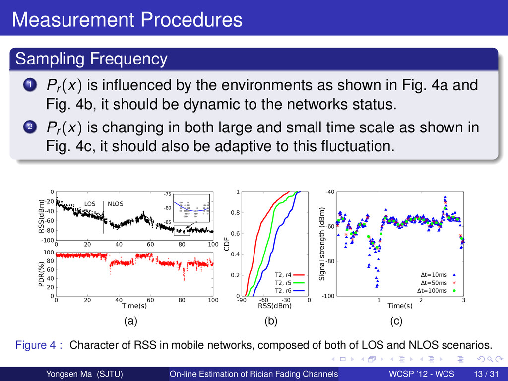
15. Measurement Procedures Sampling Frequency 1 Pr (x) is influenced by the environments as shown in Fig. 4a and Fig. 4b, it should be dynamic to the networks status. 2 Pr (x) is changing in both large and small time scale as shown in Fig. 4c, it should also be adaptive to this fluctuation. -100 -80 -60 -40 -20 0 0 20 40 60 80 100 RSS(dBm) LOS NLOS -85 -80 -75 0 20 40 60 80 100 0 20 40 60 80 100 PDR(%) Time(s) (a) 0 0.2 0.4 0.6 0.8 1 -90 -60 -30 0 CDF RSS(dBm) T2, r4 T2, r5 T2, r6 (b) -100 -80 -60 -40 1 2 3 Signal strength (dBm) Time(s) Δt=10ms Δt=50ms Δt=100ms (c) Figure 4 : Character of RSS in mobile networks, composed of both of LOS and NLOS scenarios. Yongsen Ma (SJTU) On-line Estimation of Rician Fading Channels WCSP ’12 - WCS 13 / 31
16. Outline 1 Introduction Background Propagation Models Measurement Procedures 2 On-line Estimation Measurement Framework Length of Statistical Intervals Number of Averaging Samples 3 Performance Evaluation Implementation Experiment Evaluation Yongsen Ma (SJTU) On-line Estimation of Rician Fading Channels WCSP ’12 - WCS 14 / 31
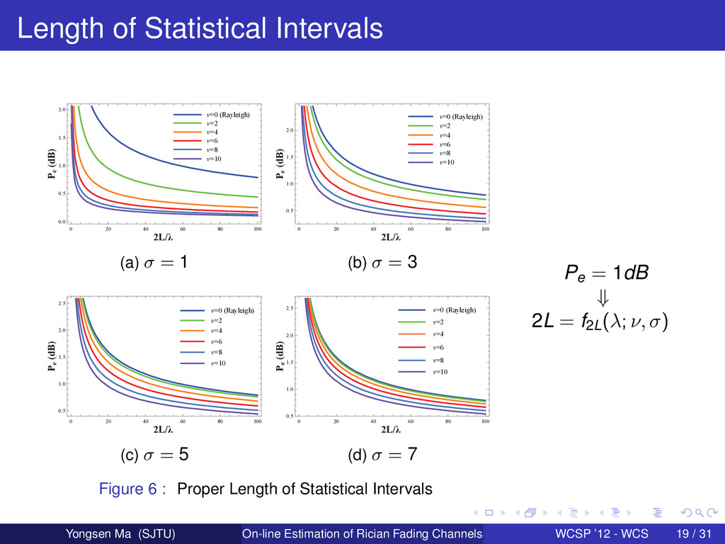
17. Measurement Framework Signal Strength Dynamic Sampling Signal Strength Dynamic Sampling Fading Parameters Dynamic Estimating Fading Parameters Dynamic Estimating Statistics Interval Statistics Interval Geographic Information System Geographic Information System Mobile Station's Speed and Direction Mobile Station's Speed and Direction Received Signal Sampling Numbers Figure 5 : On-line and Dynamic Estimation of Rician Fading Channels The on-line estimation algorithm in this paper adopts the Lee’s standard procedure in the case of Rician fading. Fig. 5 shows the basic estimation steps which mainly consist of the determination of proper length of statistical interval and required number of averaging samples. Yongsen Ma (SJTU) On-line Estimation of Rician Fading Channels WCSP ’12 - WCS 15 / 31
18. Outline 1 Introduction Background Propagation Models Measurement Procedures 2 On-line Estimation Measurement Framework Length of Statistical Intervals Number of Averaging Samples 3 Performance Evaluation Implementation Experiment Evaluation Yongsen Ma (SJTU) On-line Estimation of Rician Fading Channels WCSP ’12 - WCS 16 / 31
19. Length of Statistical Intervals ˆ s = 1 2L y+L y−L p2 r (x)dx = s 2L y+L y−L h(x)dx (4) σ2 ˆ s = 2(n − 1) n2(1 + K)2 n 0 g(K; ρ)dρ (5) Yongsen Ma (SJTU) On-line Estimation of Rician Fading Channels WCSP ’12 - WCS 17 / 31
20. Length of Statistical Intervals ˆ s = 1 2L y+L y−L p2 r (x)dx = s 2L y+L y−L h(x)dx (4) σ2 ˆ s = 2(n − 1) n2(1 + K)2 n 0 g(K; ρ)dρ (5) ⇓ Pe : = 10 log10 ˆ s + σˆ s ˆ s − σˆ s = 10 log10       n(1 + K) + 2(1 + n) n 0 g(K; ρ)dρ n(1 + K) − 2(1 + n) n 0 g(K; ρ)dρ       (6) Yongsen Ma (SJTU) On-line Estimation of Rician Fading Channels WCSP ’12 - WCS 17 / 31
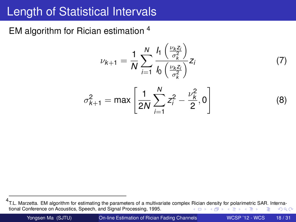
21. Length of Statistical Intervals EM algorithm for Rician estimation 4 νk+1 = 1 N N i=1 I1 νk zi σ2 k I0 νk zi σ2 k zi (7) σ2 k+1 = max 1 2N N i=1 z2 i − ν2 k 2 , 0 (8) 4 T.L. Marzetta. EM algorithm for estimating the parameters of a multivariate complex Rician density for polarimetric SAR. Interna- tional Conference on Acoustics, Speech, and Signal Processing, 1995. Yongsen Ma (SJTU) On-line Estimation of Rician Fading Channels WCSP ’12 - WCS 18 / 31
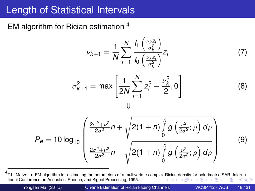
22. Length of Statistical Intervals EM algorithm for Rician estimation 4 νk+1 = 1 N N i=1 I1 νk zi σ2 k I0 νk zi σ2 k zi (7) σ2 k+1 = max 1 2N N i=1 z2 i − ν2 k 2 , 0 (8) ⇓ Pe = 10 log10       2σ2+ν2 2σ2 n + 2(1 + n) n 0 g ν2 2σ2 ; ρ dρ 2σ2+ν2 2σ2 n − 2(1 + n) n 0 g ν2 2σ2 ; ρ dρ       (9) 4 T.L. Marzetta. EM algorithm for estimating the parameters of a multivariate complex Rician density for polarimetric SAR. Interna- tional Conference on Acoustics, Speech, and Signal Processing, 1995. Yongsen Ma (SJTU) On-line Estimation of Rician Fading Channels WCSP ’12 - WCS 18 / 31
23. Length of Statistical Intervals Ν=0 (Rayleigh) Ν=10 Ν=8 Ν=6 Ν=4 Ν=2 0 20 40 60 80 100 0.0 0.5 1.0 1.5 2.0 2L Λ P_e dB Pe (dB) 2L/Ȝ (a) σ = 1 Ν=0 (Rayleigh) Ν=2 Ν=4 Ν=6 Ν=8 Ν=10 0 20 40 60 80 100 0.5 1.0 1.5 2.0 2L Λ P_e dB Pe (dB) 2L/Ȝ (b) σ = 3 Ν=0 (Rayleigh) Ν=2 Ν=10 Ν=8 Ν=6 Ν=4 0 20 40 60 80 100 0.5 1.0 1.5 2.0 2.5 2L Λ P_e dB Pe (dB) 2L/Ȝ (c) σ = 5 Ν=0 (Rayleigh) Ν=10 Ν=8 Ν=6 Ν=4 Ν=2 0 20 40 60 80 100 0.5 1.0 1.5 2.0 2.5 2L Λ P_e dB Pe (dB) 2L/Ȝ (d) σ = 7 Figure 6 : Proper Length of Statistical Intervals Pe = 1dB ⇓ 2L = f2L(λ; ν, σ) Yongsen Ma (SJTU) On-line Estimation of Rician Fading Channels WCSP ’12 - WCS 19 / 31
24. Outline 1 Introduction Background Propagation Models Measurement Procedures 2 On-line Estimation Measurement Framework Length of Statistical Intervals Number of Averaging Samples 3 Performance Evaluation Implementation Experiment Evaluation Yongsen Ma (SJTU) On-line Estimation of Rician Fading Channels WCSP ’12 - WCS 20 / 31
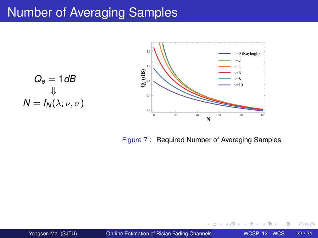
25. Number of Averaging Samples The received power r2 = 2σ2 + ν2 ≈ 1 N N i=1 z2 i can be calculated by (7) and (8), then the expectation and variance of r2 can be calculated: ¯ r2 = E r2 = 1 N E N i=1 z2 i = σ2 N 2N + ν2 (10) σ¯ r2 = D r2 = 1 N2 D N i=1 z2 i = σ4 N2 4N + 4ν2 (11) Yongsen Ma (SJTU) On-line Estimation of Rician Fading Channels WCSP ’12 - WCS 21 / 31
26. Number of Averaging Samples The received power r2 = 2σ2 + ν2 ≈ 1 N N i=1 z2 i can be calculated by (7) and (8), then the expectation and variance of r2 can be calculated: ¯ r2 = E r2 = 1 N E N i=1 z2 i = σ2 N 2N + ν2 (10) σ¯ r2 = D r2 = 1 N2 D N i=1 z2 i = σ4 N2 4N + 4ν2 (11) ⇓ Qe = 10 log10 ¯ r2 + σ¯ r2 ¯ r2 = 10 log10 σ2 N 2N + ν2 + 2σ2 N √ N + ν2 σ2 N (2N + ν2) = 10 log10 2N + ν2 + 2 √ N + ν2 2N + ν2 (12) Yongsen Ma (SJTU) On-line Estimation of Rician Fading Channels WCSP ’12 - WCS 21 / 31
27. Number of Averaging Samples Qe = 1dB ⇓ N = fN(λ; ν, σ) Ν=0 (Rayleigh) Ν=10 Ν=8 Ν=6 Ν=4 Ν=2 0 20 40 60 80 100 0.4 0.6 0.8 1.0 1.2 N Q_e dB N Qe (dB) Figure 7 : Required Number of Averaging Samples Yongsen Ma (SJTU) On-line Estimation of Rician Fading Channels WCSP ’12 - WCS 22 / 31
28. Number of Averaging Samples Qe = 1dB ⇓ N = fN(λ; ν, σ) Ν=0 (Rayleigh) Ν=10 Ν=8 Ν=6 Ν=4 Ν=2 0 20 40 60 80 100 0.4 0.6 0.8 1.0 1.2 N Q_e dB N Qe (dB) Figure 7 : Required Number of Averaging Samples ∆d = 2L/N = f2L (λ; ν, σ)/fN (λ; ν, σ) = fd (λ; ν, σ) ∆d ⇐ statistical interval 2L and number of averaging samples N; ∆d ⇒ measurement accuracy and overhead of on-line estimation. Yongsen Ma (SJTU) On-line Estimation of Rician Fading Channels WCSP ’12 - WCS 22 / 31
29. Outline 1 Introduction Background Propagation Models Measurement Procedures 2 On-line Estimation Measurement Framework Length of Statistical Intervals Number of Averaging Samples 3 Performance Evaluation Implementation Experiment Evaluation Yongsen Ma (SJTU) On-line Estimation of Rician Fading Channels WCSP ’12 - WCS 23 / 31
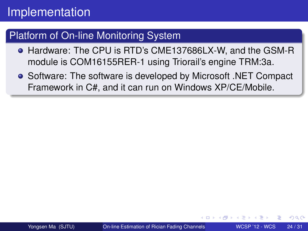
30. Implementation Platform of On-line Monitoring System Hardware: The CPU is RTD’s CME137686LX-W, and the GSM-R module is COM16155RER-1 using Triorail’s engine TRM:3a. Software: The software is developed by Microsoft .NET Compact Framework in C#, and it can run on Windows XP/CE/Mobile. Yongsen Ma (SJTU) On-line Estimation of Rician Fading Channels WCSP ’12 - WCS 24 / 31
31. Implementation Platform of On-line Monitoring System Hardware: The CPU is RTD’s CME137686LX-W, and the GSM-R module is COM16155RER-1 using Triorail’s engine TRM:3a. Software: The software is developed by Microsoft .NET Compact Framework in C#, and it can run on Windows XP/CE/Mobile. (a) Hardware Design (b) Software Development Figure 8 : Um Interface Monitoring System for GSM-R Networks Yongsen Ma (SJTU) On-line Estimation of Rician Fading Channels WCSP ’12 - WCS 24 / 31
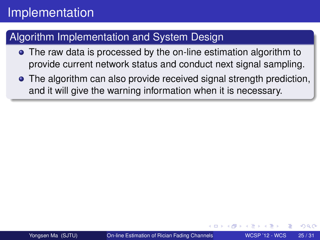
32. Implementation Algorithm Implementation and System Design The raw data is processed by the on-line estimation algorithm to provide current network status and conduct next signal sampling. The algorithm can also provide received signal strength prediction, and it will give the warning information when it is necessary. Yongsen Ma (SJTU) On-line Estimation of Rician Fading Channels WCSP ’12 - WCS 25 / 31
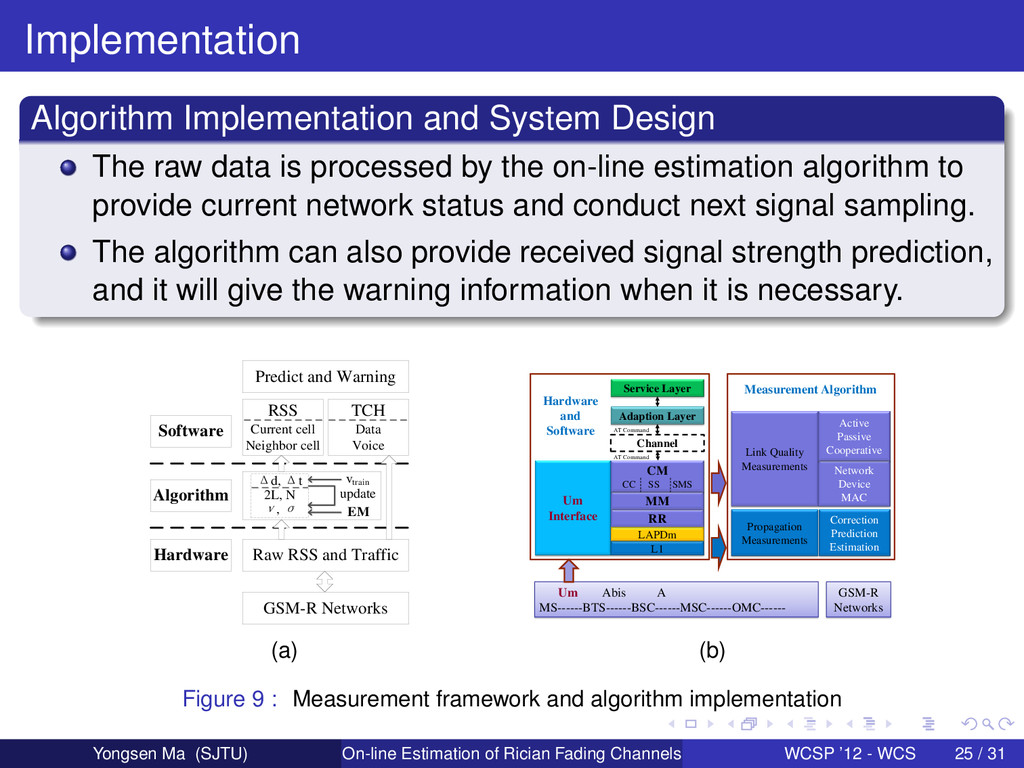
33. Implementation Algorithm Implementation and System Design The raw data is processed by the on-line estimation algorithm to provide current network status and conduct next signal sampling. The algorithm can also provide received signal strength prediction, and it will give the warning information when it is necessary. Hardware Algorithm Software RSS Current cell Neighbor cell TCH Data Voice Predict and Warning Raw RSS and Traffic GSM-R Networks Δd, Δt 2L, N ν, σ vtrain EM update (a) GSM-R Networks Um Abis A MS------BTS------BSC------MSC------OMC------ Propagation Measurements Correction Prediction Estimation Um Interface L1 LAPDm RR MM CM CC SS SMS Channel Adaption Layer Service Layer AT Command AT Command Link Quality Measurements Network Device MAC Active Passive Cooperative Hardware and Software Measurement Algorithm (b) Figure 9 : Measurement framework and algorithm implementation Yongsen Ma (SJTU) On-line Estimation of Rician Fading Channels WCSP ’12 - WCS 25 / 31
34. Outline 1 Introduction Background Propagation Models Measurement Procedures 2 On-line Estimation Measurement Framework Length of Statistical Intervals Number of Averaging Samples 3 Performance Evaluation Implementation Experiment Evaluation Yongsen Ma (SJTU) On-line Estimation of Rician Fading Channels WCSP ’12 - WCS 26 / 31
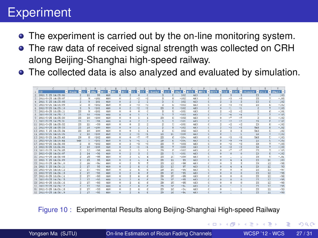
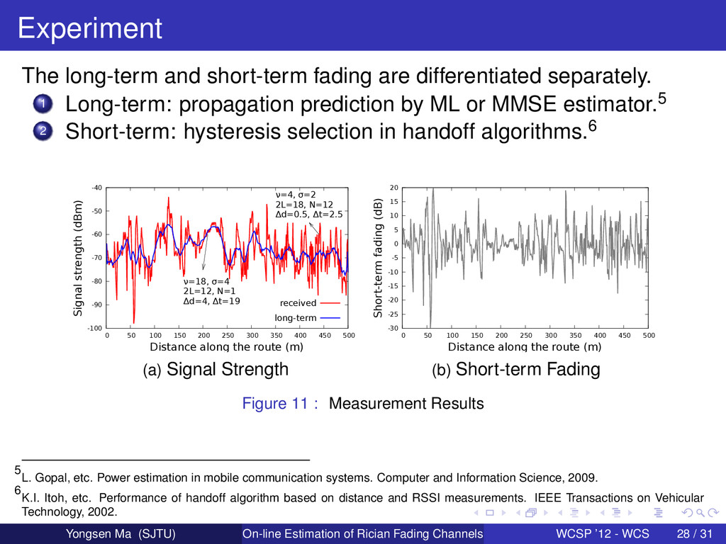
35. Experiment The experiment is carried out by the on-line monitoring system. The raw data of received signal strength was collected on CRH along Beijing-Shanghai high-speed railway. The collected data is also analyzed and evaluated by simulation. Figure 10 : Experimental Results along Beijing-Shanghai High-speed Railway Yongsen Ma (SJTU) On-line Estimation of Rician Fading Channels WCSP ’12 - WCS 27 / 31
36. Experiment The long-term and short-term fading are differentiated separately. 1 Long-term: propagation prediction by ML or MMSE estimator.5 2 Short-term: hysteresis selection in handoff algorithms.6 -100 -90 -80 -70 -60 -50 -40 0 50 100 150 200 250 300 350 400 450 500 Signal strength (dBm) Distance along the route (m) ν=18, σ=4 2L=12, N=1 Δd=4, Δt=19 ν=4, σ=2 2L=18, N=12 Δd=0.5, Δt=2.5 received long-term (a) Signal Strength -30 -25 -20 -15 -10 -5 0 5 10 15 20 0 50 100 150 200 250 300 350 400 450 500 Short-term fading (dB) Distance along the route (m) (b) Short-term Fading Figure 11 : Measurement Results 5 L. Gopal, etc. Power estimation in mobile communication systems. Computer and Information Science, 2009. 6 K.I. Itoh, etc. Performance of handoff algorithm based on distance and RSSI measurements. IEEE Transactions on Vehicular Technology, 2002. Yongsen Ma (SJTU) On-line Estimation of Rician Fading Channels WCSP ’12 - WCS 28 / 31
37. Outline 1 Introduction Background Propagation Models Measurement Procedures 2 On-line Estimation Measurement Framework Length of Statistical Intervals Number of Averaging Samples 3 Performance Evaluation Implementation Experiment Evaluation Yongsen Ma (SJTU) On-line Estimation of Rician Fading Channels WCSP ’12 - WCS 29 / 31
38. Evaluation ∆d is more larger compared to Lee’s method when K = 0, which means the multi-path fading is Rayleigh distributed. ∆d may be not so small although 2L decreases, for n < 5 when the terrains gradually become flat until ν > 10. Table 1 : Summary of Experiment Results Terrain K(dB) ν σ 2L(λ) N ∆d(λ) ∆d(m) vtrain (km/h) 200 250 300 ∆t(ms) NLOS* 0 - - 40 36 1.1 0.367 2.20 1.76 1.47 Intensive 0 0 1 55 15 3.7 1.222 7.33 5.86 4.89 2 4 2 18 12 1.5 0.500 3.00 2.40 2.00 4 5.6 2 9 9 1.0 0.333 2.00 1.60 1.33 6 6 3 20 7 2.9 0.967 5.80 4.64 3.87 8 12 3 8 1 8.0 2.667 16.00 12.80 10.67 Open 10 18 4 12 1 12.0 4.000 24.00 19.20 16.00 * Caculated by Lee’s method in the case of Rayleigh fading Yongsen Ma (SJTU) On-line Estimation of Rician Fading Channels WCSP ’12 - WCS 30 / 31
39. On-line Estimation of Rician Fading Channels THANKS! Yongsen Ma (SJTU) On-line Estimation of Rician Fading Channels WCSP ’12 - WCS 31 / 31