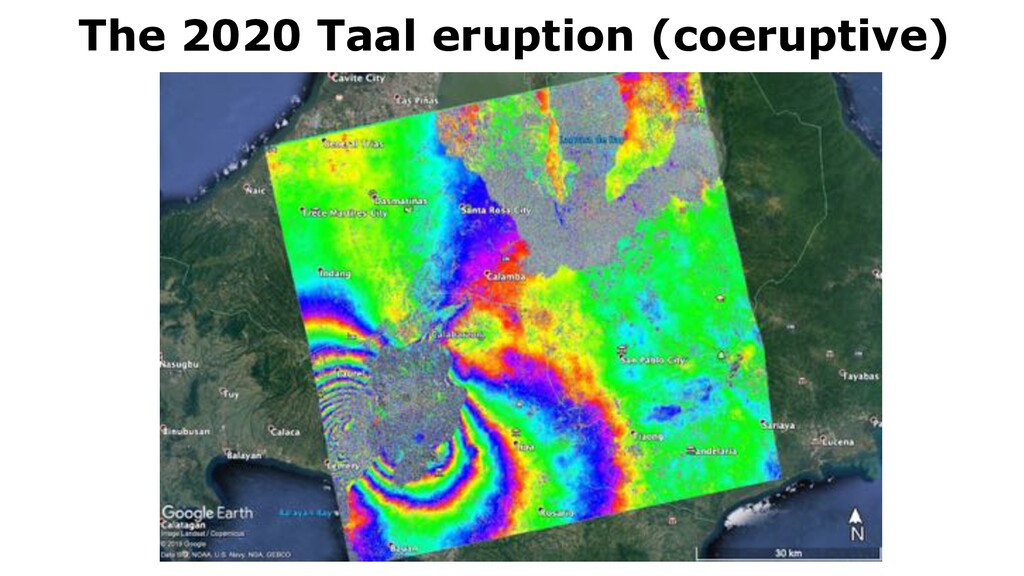
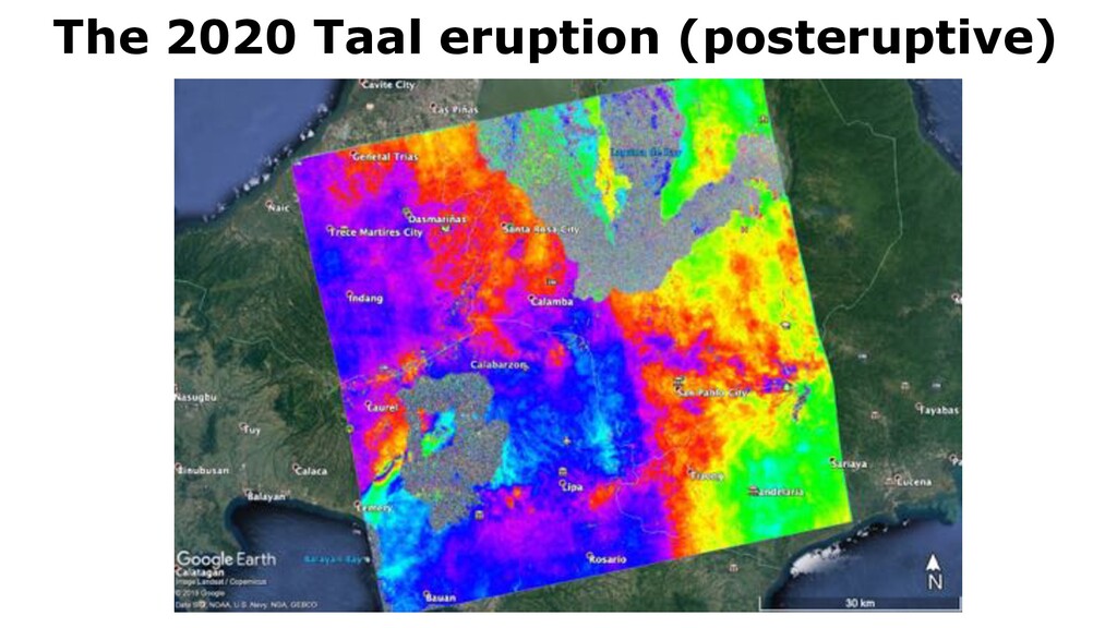
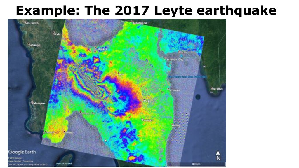
Processing Stripmap SAR images 2-a Deformation of the 2017 Leyte earthquake 2-b Deformation of the 2019 Luzon earthquake 2-c Deformation of the 2020 Taal eruption 3. Damage detection from SAR images 2-a The 2017 Leyte earthquake 2-b The 2020 Taal eruption 4. Processing ScanSAR images 4-a. The 2019 Cotabato and Davao del Sur (Mindanao) earthquakes 4-b. The 2020 Taal eruption
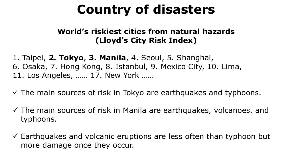
hazards (Lloyd’s City Risk Index) 1. Taipei, 2. Tokyo, 3. Manila, 4. Seoul, 5. Shanghai, 6. Osaka, 7. Hong Kong, 8. Istanbul, 9. Mexico City, 10. Lima, 11. Los Angeles, …… 17. New York …… ü The main sources of risk in Tokyo are earthquakes and typhoons. ü The main sources of risk in Manila are earthquakes, volcanoes, and typhoons. ü Earthquakes and volcanic eruptions are less often than typhoon but more damage once they occur.
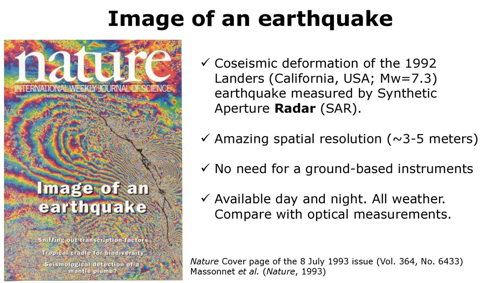
July 1993 issue (Vol. 364, No. 6433) Massonnet et al. (Nature, 1993) ü Coseismic deformation of the 1992 Landers (California, USA; Mw=7.3) earthquake measured by Synthetic Aperture Radar (SAR). ü Amazing spatial resolution (~3-5 meters) ü No need for a ground-based instruments ü Available day and night. All weather. Compare with optical measurements.
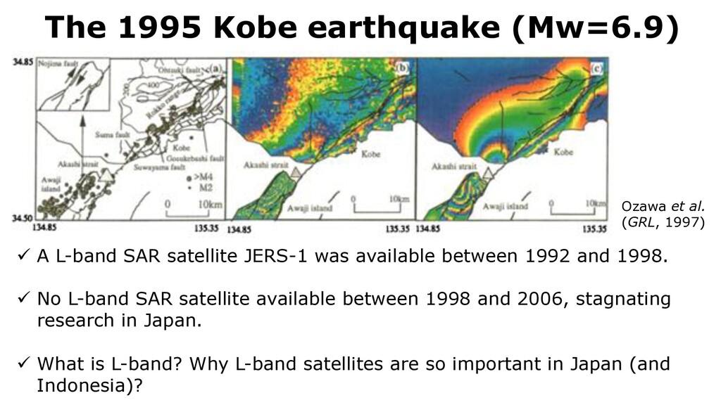
example, the deformation due to the 1995 Kobe earthquake was measured by InSAR (Ozawa et al., 1997; Fig. 2). In spite of this worldwide trend, however, InSAR studies did Figure 2: An interferogram associated with the 1995 Kobe earthquake. (a) Aftershock distribution due the Kobe earthquake. Triangle denotes the epicenter of the mainshock. (b) Observed coseismic deformation. (c) Calculated deformation from a fault model. Taken from Ozawa et al., (1997). not become very popular among Japanese scientists mainly because of the lack of a satellite with a long wavelength (L-band) which is required to measure deformation in vegetated regions such as the Japanese islands. JERS-1, a L-band satellite, ended its operation in 1998. Ozawa et al. (GRL, 1997) ü A L-band SAR satellite JERS-1 was available between 1992 and 1998. ü No L-band SAR satellite available between 1998 and 2006, stagnating research in Japan. ü What is L-band? Why L-band satellites are so important in Japan (and Indonesia)?
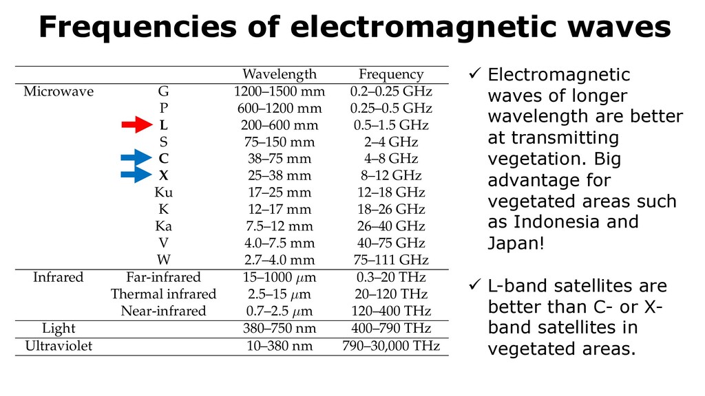
0.2–0.25 GHz P 600–1200 mm 0.25–0.5 GHz L 200–600 mm 0.5–1.5 GHz S 75–150 mm 2–4 GHz C 38–75 mm 4–8 GHz X 25–38 mm 8–12 GHz Ku 17–25 mm 12–18 GHz K 12–17 mm 18–26 GHz Ka 7.5–12 mm 26–40 GHz V 4.0–7.5 mm 40–75 GHz W 2.7–4.0 mm 75–111 GHz Infrared Far-infrared 15–1000 µm 0.3–20 THz Thermal infrared 2.5–15 µm 20–120 THz Near-infrared 0.7–2.5 µm 120–400 THz Light 380–750 nm 400–790 THz Ultraviolet 10–380 nm 790–30,000 THz ü Electromagnetic waves of longer wavelength are better at transmitting vegetation. Big advantage for vegetated areas such as Indonesia and Japan! ü L-band satellites are better than C- or X- band satellites in vegetated areas.
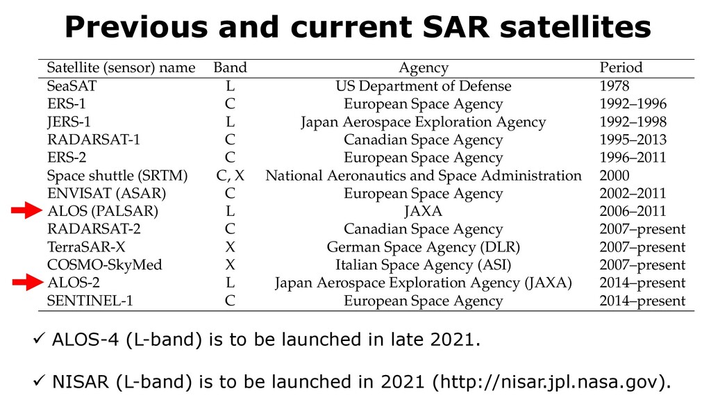
Period SeaSAT L US Department of Defense 1978 ERS-1 C European Space Agency 1992–1996 JERS-1 L Japan Aerospace Exploration Agency 1992–1998 RADARSAT-1 C Canadian Space Agency 1995–2013 ERS-2 C European Space Agency 1996–2011 Space shuttle (SRTM) C, X National Aeronautics and Space Administration 2000 ENVISAT (ASAR) C European Space Agency 2002–2011 ALOS (PALSAR) L JAXA 2006–2011 RADARSAT-2 C Canadian Space Agency 2007–present TerraSAR-X X German Space Agency (DLR) 2007–present COSMO-SkyMed X Italian Space Agency (ASI) 2007–present ALOS-2 L Japan Aerospace Exploration Agency (JAXA) 2014–present SENTINEL-1 C European Space Agency 2014–present Table 2: SAR satellites launched so far. ü ALOS-4 (L-band) is to be launched in late 2021. ü NISAR (L-band) is to be launched in 2021 (http://nisar.jpl.nasa.gov).
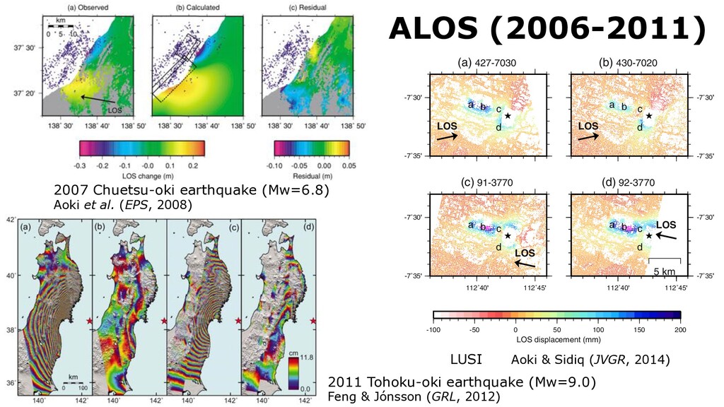
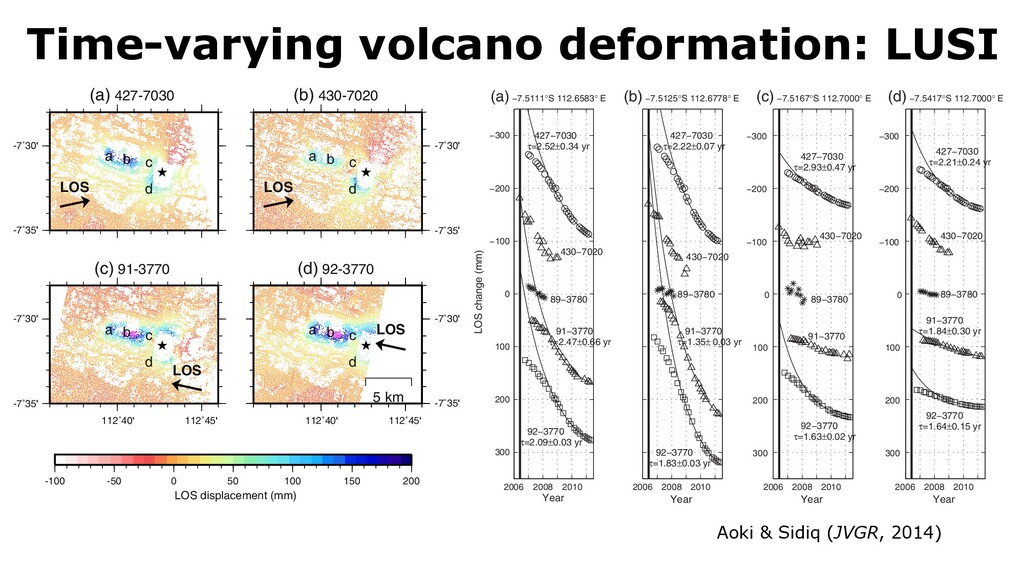
(Aoki et al., 2008). Blue dots denote of aftershocks. (a) Observed changes of line-of sight shown by an arrow. Note that vertical i) east-west displacements cannot be separated. Gray depicts incoherent areas mainly due all. (b) Calculated displacement field by a fault model. (c) Residual between observed and displacements. 3 The derived relaxation times do not vary much between western and eastern points; they are mostly between 1.5 and 2.5 years (Fig. 4). Note that a relaxation time is estimated only when an F-test (e.g., Menke, 2012, pp. 111–112) shows that the time series better than a linear fit with a relaxation time is not obtained from noisy or -7˚35 -7˚30 (a) 427-7030 a b c d LOS -7˚35 -7˚30 (b) 430-7020 a b c d LOS 112˚40 112˚45 -7˚35 -7˚30 (c) 91-3770 a b c d LOS 112˚40 -7˚35 -7˚30 (d) 92-3770 a b c d LOS 112˚45 5 km -100 -50 0 50 100 150 200 LOS displacement (mm) -7˚30 (e) 89-3780 2007 Chuetsu-oki earthquake (Mw=6.8) Aoki et al. (EPS, 2008) 2011 Tohoku-oki earthquake (Mw=9.0) Feng & Jónsson (GRL, 2012) LUSI Aoki & Sidiq (JVGR, 2014)
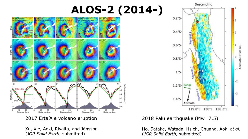
Chuang, Aoki et al. (JGR Solid Earth, submitted) 2017 Erta’Ale volcano eruption Xu, Xie, Aoki, Rivalta, and Jónsson (JGR Solid Earth, submitted) 167 Figure 3. Azimuth offsets from (a) descending (S 168 observed by Sentinel-1. The red stars show the 169 green arrows indicate the azimuth and range direc 170 2.3 Tsunami Waveform 171 7 from the southern caldera (Fig. 3). 145 146 147
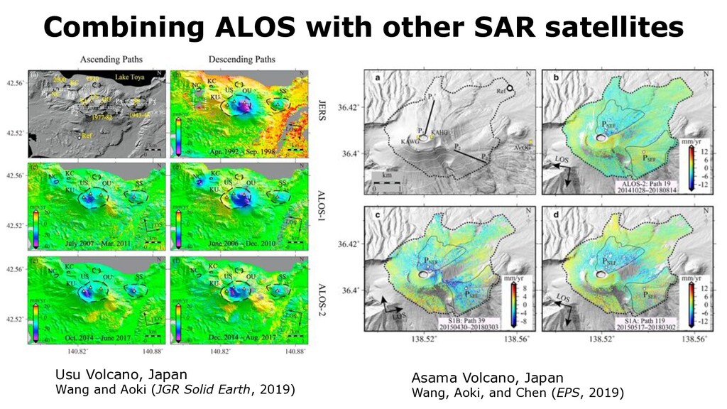
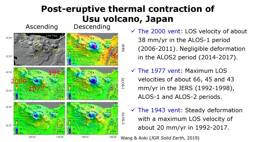
Aoki, and Chen (EPS, 2019) Usu Volcano, Japan Wang and Aoki (JGR Solid Earth, 2019) Figure 5. (a) The digital elevation model used in the interferometric synthetic aperture radar processing. The black dashed polygons represent vents of the previous eruptions. P1P1′, P2P2′, and P3P3′ are profiles across the 2000, 1977, and 1943 eruption sites, respectively. (b) Mean line‐of‐sight velocities derived from JERS images using the stacking method. The white rectangle indicates the masked region due to large topographic errors. (c, d) Mean LOS velocities derived from the small baseline subset processing of ascending and descending ALOS‐1 images. (e, f) Mean line‐of‐sight 10.1029/2018JB016729 al of Geophysical Research: Solid Earth Page 9 of 16 Wang et al. Earth, Planets and Space (2019) 71:121 Fig. 7 a Topography around Asama volcano. Two solid lines indicate profiles whose LOS displacements are shown in Fig. 8. The mean LOS velocities from the b ALOS-2, c ascending Sentinel-1, and d descending Sentinel-1 images. Two deformation regions at the northeast and southeast of the volcano are circled by solid black lines in b‒d. PNEF and PSEF are the two points selected for plotting the displacement time series in Fig. 9. Black dotted lines in all panels indicate the area with NDVI value smaller than 0.4 as shown in Fig. 2b. The time span in each sub-figure indicates the observation period
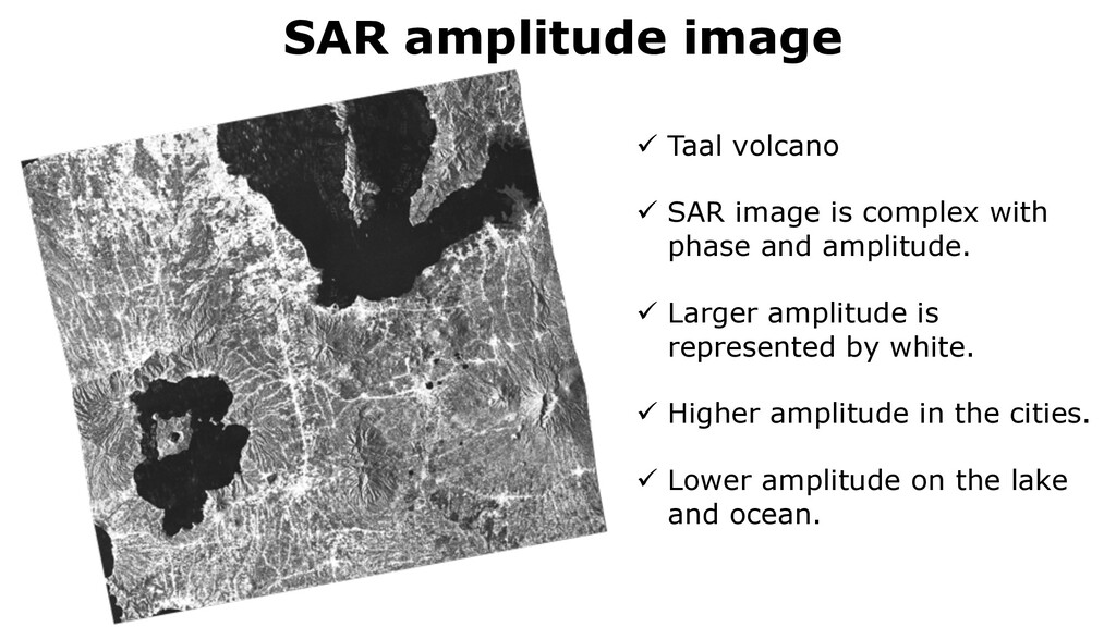
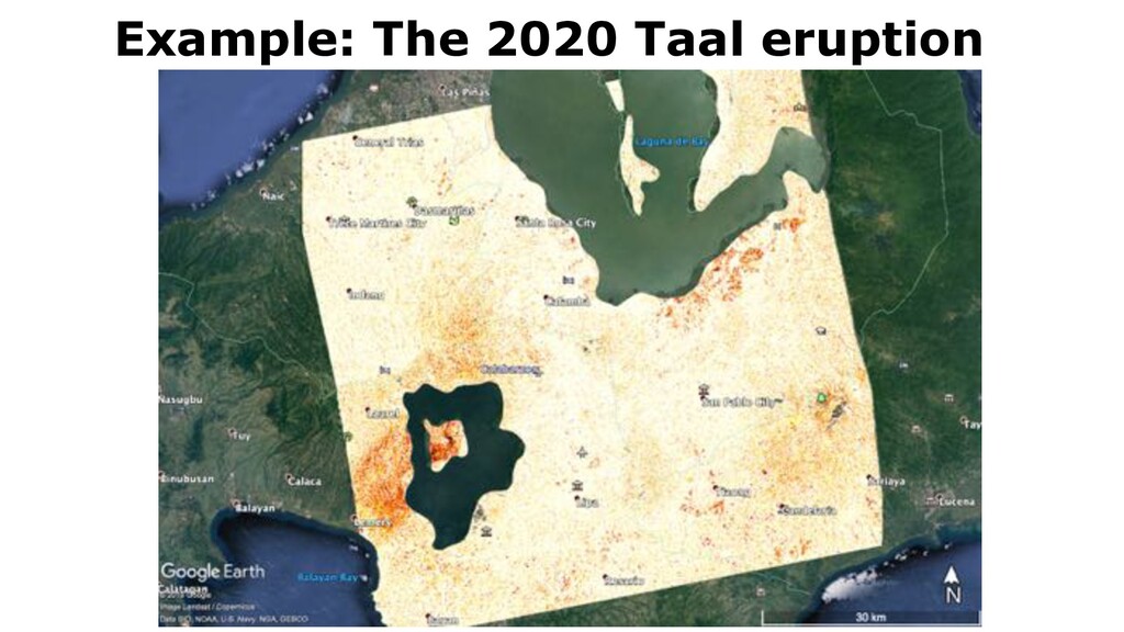
complex with phase and amplitude. ü Larger amplitude is represented by white. ü Higher amplitude in the cities. ü Lower amplitude on the lake and ocean.
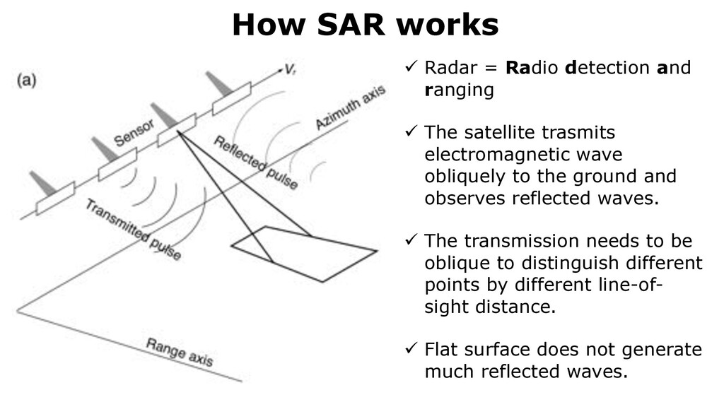
flight of the satellite is called ”azimuth” and the dir is the emission of microwaves is called ”range” (Fig. 8). A SAR sensor emits pulses of microw ü Radar = Radio detection and ranging ü The satellite trasmits electromagnetic wave obliquely to the ground and observes reflected waves. ü The transmission needs to be oblique to distinguish different points by different line-of- sight distance. ü Flat surface does not generate much reflected waves.
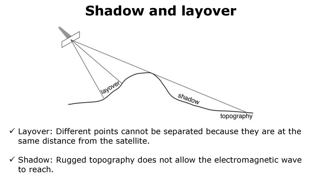
By the way, microw matic view of layover and shadow resulting from an oblique incidence o pography. ü Layover: Different points cannot be separated because they are at the same distance from the satellite. ü Shadow: Rugged topography does not allow the electromagnetic wave to reach.
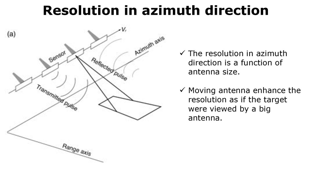
is a function of antenna size. ü Moving antenna enhance the resolution as if the target were viewed by a big antenna. h’s surface. By convention, the direction of flight of the satellite is called ”azimuth” and the dir is the emission of microwaves is called ”range” (Fig. 8). A SAR sensor emits pulses of microw
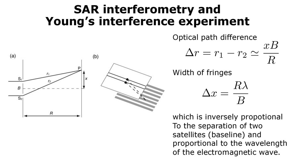
interference experiment. (b) An extension of (a) to three ellite orbits in two different timings are denoted by black lines dots. the point P in Fig. 13a, redoubling the strength or destroying each other depending r = r1 r2 ' xB R x = R B Optical path difference Width of fringes which is inversely propotional To the separation of two satellites (baseline) and proportional to the wavelength of the electromagnetic wave.
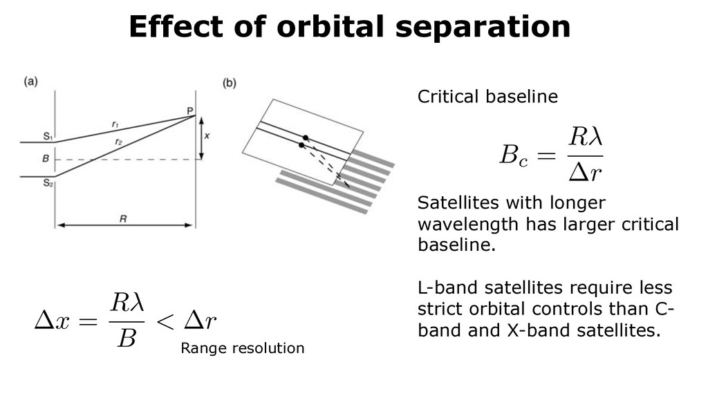
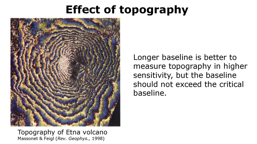
(b) An extension of (a) to three ellite orbits in two different timings are denoted by black lines dots. the point P in Fig. 13a, redoubling the strength or destroying each other depending ath difference. This results in fringes on the wall. When R x ± d/2, The optical path r1 − r2 (Fig. 13a) is given by Critical baseline Satellites with longer wavelength has larger critical baseline. L-band satellites require less strict orbital controls than C- band and X-band satellites. x = R B < r Range resolution Bc = R r
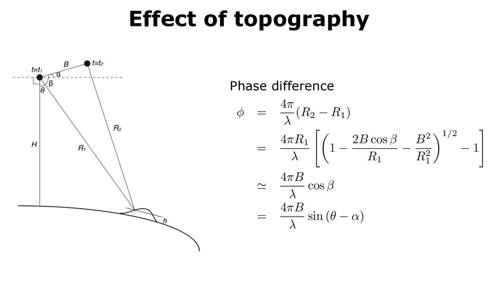
= 4π λ (R2 − R1 ) = 4πR1 λ 1 − 2B cos β R1 − B2 R2 1 1/2 − 1 4πB λ cos β = 4πB λ sin (θ − α) where λ is the wavelength of microwave and R1 and R2 represent satellite t1 and t2 , respectively. An approximation from equation (??) to (??) is due Phase difference
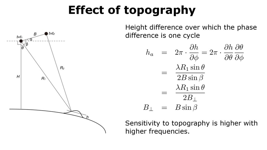
is one cycle Sensitivity to topography is higher with higher frequencies. where λ is the wavelength of microwave and R1 and R2 represent sate t1 and t2 , respectively. An approximation from equation (??) to (??) is β = π/2 − (θ − α). Equation (25) and h = H − R1 cos θ gives the height phase shift is one cycle or 2π as ha = 2π · ∂h ∂φ = 2π · ∂h ∂θ ∂θ ∂φ = λR1 sin θ 2B sin β = λR1 sin θ 2B⊥ B⊥ = B sin β Smaller ha , more sensitive to topography. Equation (26) also indicates sensitive to topography than a L-band SAR because of the shorter wavele
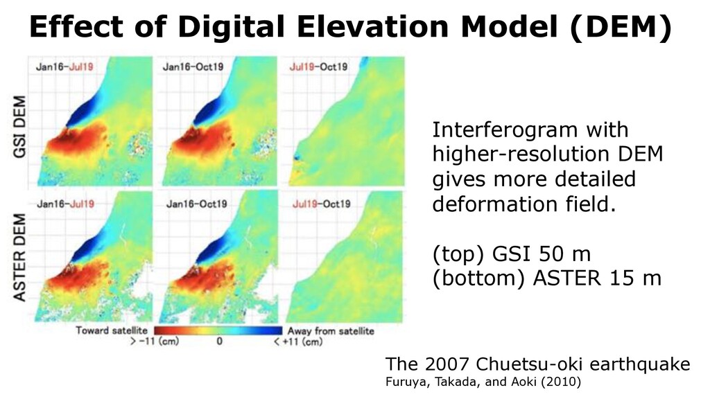
Furuya, Takada, and Aoki (2010) Interferogram with higher-resolution DEM gives more detailed deformation field. (top) GSI 50 m (bottom) ASTER 15 m erferograms with different DEMs. The upper panel shows the one with GSI DEM with
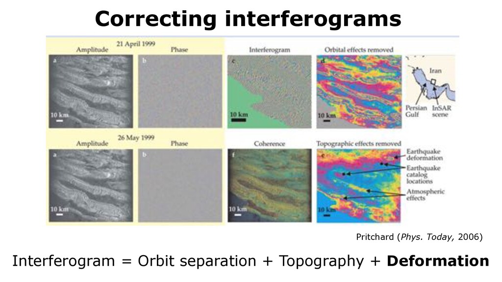
from Pritchard (2006). (a)(b) Two SLC images to gen- erate an interferogram. (c) An interferogram without corrections. (d) An interferogram after removing an orbital effect. (e) The final interferogram after removing topographical effects as well. (f) Coherence Interferogram = Orbit separation + Topography + Deformation Pritchard (Phys. Today, 2006)
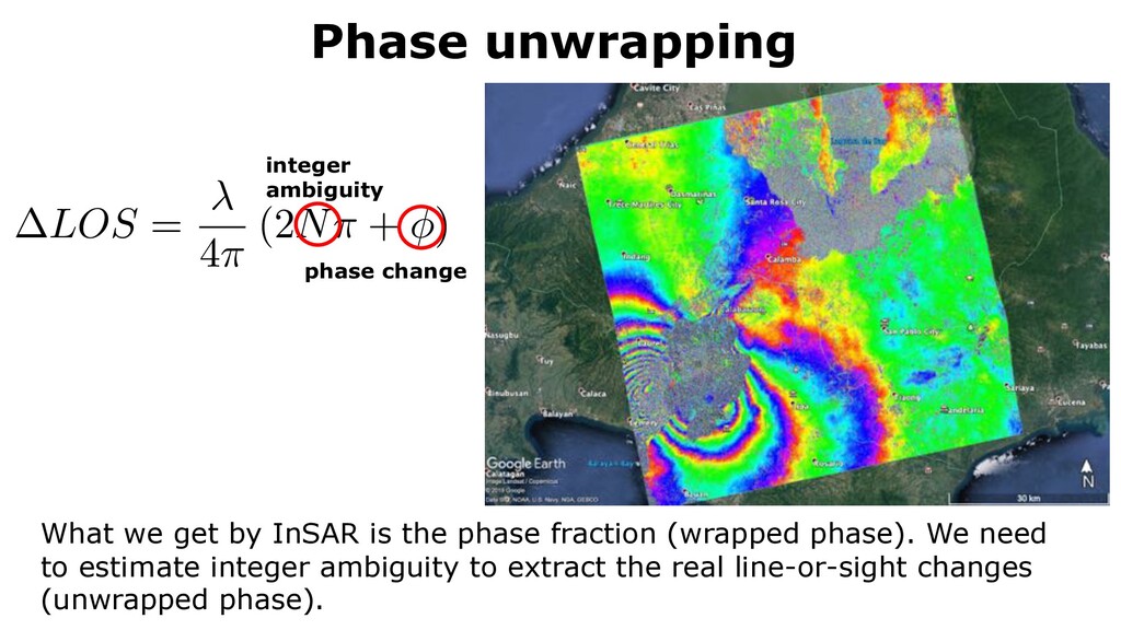
integer ambiguity What we get by InSAR is the phase fraction (wrapped phase). We need to estimate integer ambiguity to extract the real line-or-sight changes (unwrapped phase).
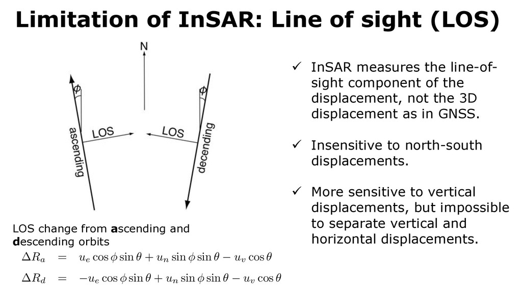
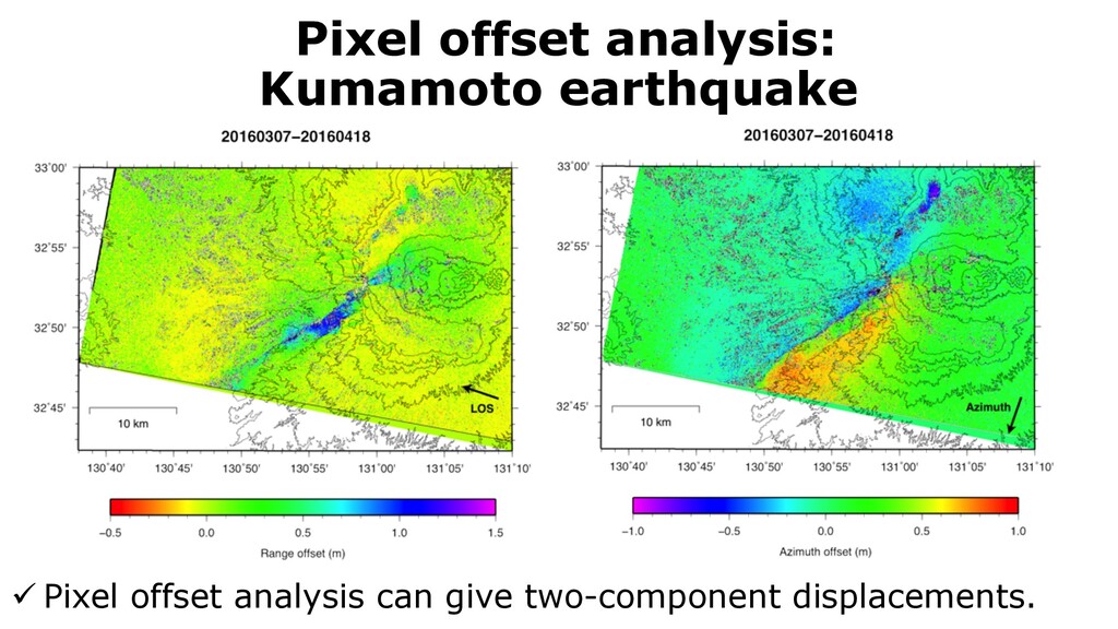
Figs. 4 and 5 may be more natural but it tends to lose small-scale deformation. nSAR s ons measure all three component displacements, InSAR measures a single com- ch pixel. Sensitivity of LOS to the three component displacement depends on taken from the ascending or descending orbit. The satellite flies from roughly ascending orbit and the other way around in the descending orbit (Fig. 18) . The ht-looking SAR satellite such as ALOS and many others is roughly from west to ng orbit and from east to west from the descending orbit. When the orbit is offset a degree of φ (Fig. 18), the LOS change is written by ∆Ra = ue cos φ sin θ + un sin φ sin θ − uv cos θ (28) ∆Rd = −ue cos φ sin θ + un sin φ sin θ − uv cos θ (29) ending orbits of the satellit. LOS is for a right-looking SAR satellit ü InSAR measures the line-of- sight component of the displacement, not the 3D displacement as in GNSS. ü Insensitive to north-south displacements. ü More sensitive to vertical displacements, but impossible to separate vertical and horizontal displacements. LOS change from ascending and descending orbits
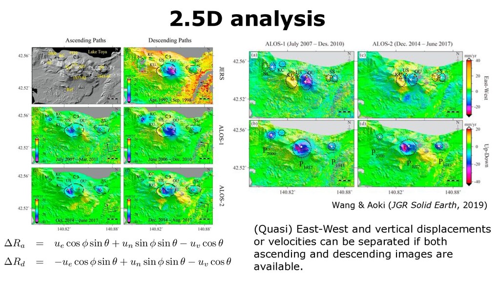
obtain the LOS displacement itself. ments themselves like Figs. 4 and 5 may be more natural but it tends to lose mall-scale deformation. AR measure all three component displacements, InSAR measures a single com- pixel. Sensitivity of LOS to the three component displacement depends on ken from the ascending or descending orbit. The satellite flies from roughly ending orbit and the other way around in the descending orbit (Fig. 18) . The ooking SAR satellite such as ALOS and many others is roughly from west to orbit and from east to west from the descending orbit. When the orbit is offset gree of φ (Fig. 18), the LOS change is written by ∆Ra = ue cos φ sin θ + un sin φ sin θ − uv cos θ (28) ∆Rd = −ue cos φ sin θ + un sin φ sin θ − uv cos θ (29) Figure 5. (a) The digital elevation model used in the interferometric synthetic aperture radar processing. The black dashed polygons represent vents of the previous eruptions. P1P1′, P2P2′, and P3P3′ are profiles across the 2000, 1977, and 1943 eruption sites, respectively. (b) Mean line‐of‐sight velocities derived from JERS images using the stacking method. The white rectangle indicates the masked region due to large topographic errors. (c, d) Mean LOS velocities derived from the small baseline subset processing of ascending and descending ALOS‐1 images. (e, f) Mean line‐of‐sight velocities obtained from the SBAS processing of ascending and descending ALOS‐2 images. The time span in each sub- figure indicates the observation period. The yellow triangles represent the dome summits that are the same as those in Figure 1. NC = Nishiyama Crater; KC = Konpirayama Crater; KU = Ko‐Usu; OU = O‐Usu; US = Usu‐Shinzan; 10.1029/2018JB016729 urnal of Geophysical Research: Solid Earth The 1977 eruption site exhibits substantial posteruptive subsidence in all the five LOS velocity maps (Figures 5b–5f). The subsidence is mainly centered at the summit crater with the deformation area extending Figure 6. Quasi east‐west and vertical displacement velocities derived from the ALOS‐1 and ALOS‐2 images. (a, b) East‐ west and vertical components from the ALOS‐1 data. (c, d) East‐west and vertical components from the ALOS‐2 data. The white arrows in (a) and (c) represent the displacement directions. P2000, P1977, and P1943 in (b) and (d) indicate points where deformation rates are shown in Table 3. The time periods in the upper annotations indicate the span the synthetic aperture radar (SAR) images involved for the calculation. The yellow triangles represent the dome summits that are the same as those in Figure 1. NC = Nishiyama Crater; KC = Konpirayama Crater; KU = Ko‐Usu; OU = O‐Usu; US = Usu‐ Shinzan; SS = Showa‐Shinzan. 10.1029/2018JB016729 Journal of Geophysical Research: Solid Earth (Quasi) East-West and vertical displacements or velocities can be separated if both ascending and descending images are available. Wang & Aoki (JGR Solid Earth, 2019)
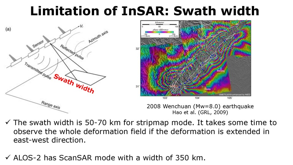
to generate a SLC image. SAR satellites take a orbit 600–800 km above th’s surface. By convention, the direction of flight of the satellite is called ”azimuth” and the direc- is the emission of microwaves is called ”range” (Fig. 8). A SAR sensor emits pulses of microwave ure 8: (a) Geometry of the observation by a SAR satellite. A target is seen only when it is within w of the satellite. (b) Center of microwave emission, denoted by a thick line is not perpendicular to direction of flight but offset by an angle of θs . length of 0.02–0.04 milliseconds every 0.5–1 milliseconds, or a frequency of 1000–2000 Hz, to the ge direction with an incident angle of 20–50 degrees from vertical. It travels to the azimuth direction Swath width Figure 19: An interferogram associated with the 2008 Wenchan earthquake obtained by SAR images from the ALOS satellite. One cycle of fringes corresponds to LOS changes of about 118 millimeters. Taken from Hao et al. (2009). 2008 Wenchuan (Mw=8.0) earthquake Hao et al. (GRL, 2009) ü The swath width is 50-70 km for stripmap mode. It takes some time to observe the whole deformation field if the deformation is extended in east-west direction. ü ALOS-2 has ScanSAR mode with a width of 350 km.
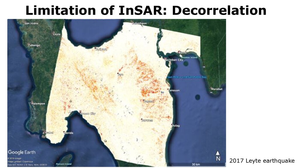
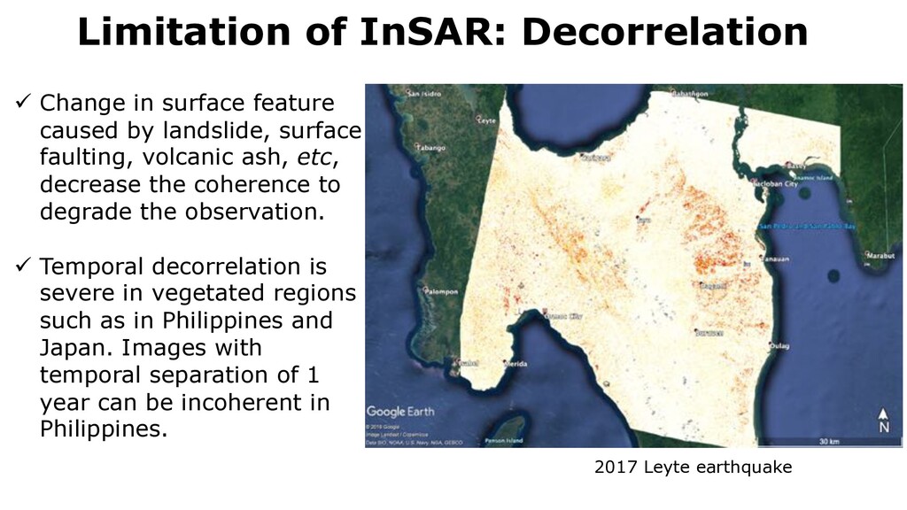
surface feature caused by landslide, surface faulting, volcanic ash, etc, decrease the coherence to degrade the observation. ü Temporal decorrelation is severe in vegetated regions such as in Philippines and Japan. Images with temporal separation of 1 year can be incoherent in Philippines.
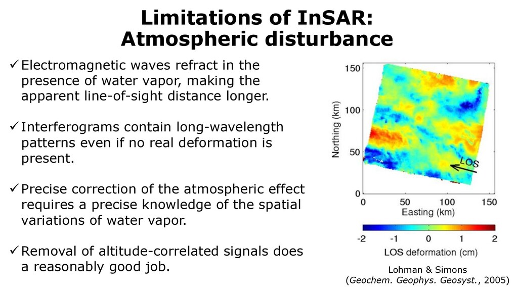
the presence of water vapor, making the apparent line-of-sight distance longer. ü Interferograms contain long-wavelength patterns even if no real deformation is present. ü Precise correction of the atmospheric effect requires a precise knowledge of the spatial variations of water vapor. ü Removal of altitude-correlated signals does a reasonably good job. Lohman & Simons (Geochem. Geophys. Geosyst., 2005)
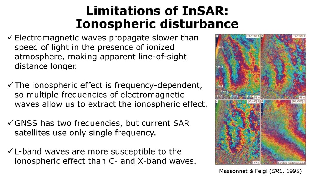
experiment with SIR-C did not detect ionospheric effects (Rosen et al., 1998). Th of the lower altitude of the SIR-C satellite (∼220 km) than other satellites so that t underestimated. Interferograms associated with the 1992 Landers earthquake (F patterns due to the ionospheric effects (Fig. 22a, b, c). Acquisition time with resp ü Electromagnetic waves propagate slower than speed of light in the presence of ionized atmosphere, making apparent line-of-sight distance longer. ü The ionospheric effect is frequency-dependent, so multiple frequencies of electromagnetic waves allow us to extract the ionospheric effect. ü GNSS has two frequencies, but current SAR satellites use only single frequency. ü L-band waves are more susceptible to the ionospheric effect than C- and X-band waves.
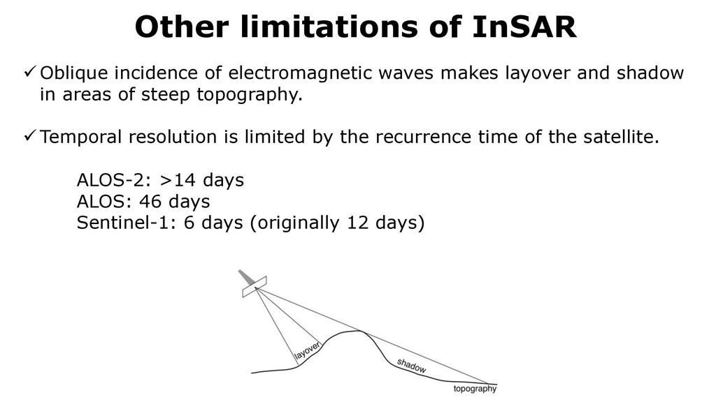
makes layover and shadow in areas of steep topography. ü Temporal resolution is limited by the recurrence time of the satellite. ALOS-2: >14 days ALOS: 46 days Sentinel-1: 6 days (originally 12 days) Figure 8: (a) Geometry of the observation by a SAR satellite. A target is seen only when it is within view of the satellite. (b) Center of microwave emission, denoted by a thick line is not perpendicular to the direction of flight but offset by an angle of θs . of a length of 0.02–0.04 milliseconds every 0.5–1 milliseconds, or a frequency of 1000–2000 Hz, to the range direction with an incident angle of 20–50 degrees from vertical. It travels to the azimuth direction by emitting microwaves and receiving back-scattered waves (Fig. 8). Note that microwaves emitting to a flat surface such as sea surface or an runway reflect forward much more than backward, resulting in a very weak signal received by the SAR sensor. In addition, an oblique incidence of microwaves yields invisible targets (called ”shadow”) or different targets with the same range distance, resulting in a skewed image (called ”foreshortening” or ”layover”) (Fig. 9). By the way, microwaves must be
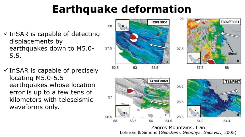
5 earthquake in Zagros Mountains, Iran, derived b Zagros Mountains, Iran Lohman & Simons (Geochem. Geophys. Geosyst., 2005) ü InSAR is capable of detecting displacements by earthquakes down to M5.0- 5.5. ü InSAR is capable of precisely locating M5.0-5.5 earthquakes whose location error is up to a few tens of kilometers with teleseismic waveforms only.
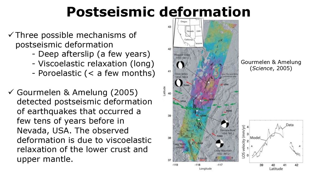
mechanisms of postseismic deformation - Deep afterslip (a few years) - Viscoelastic relaxation (long) - Poroelastic (< a few months) ü Gourmelen & Amelung (2005) detected postseismic deformation of earthquakes that occurred a few tens of years before in Nevada, USA. The observed deformation is due to viscoelastic relaxation of the lower crust and upper mantle.
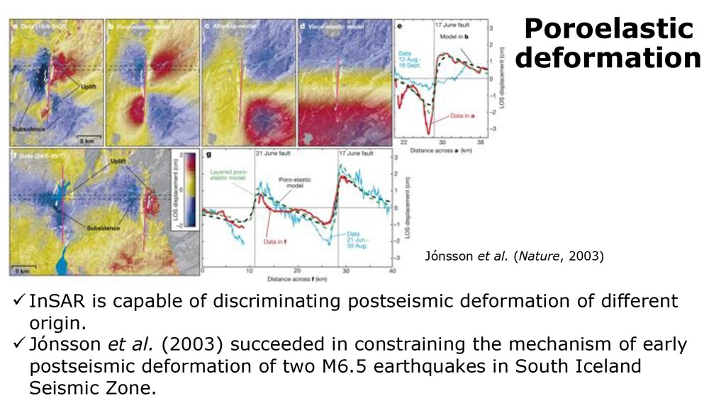
on 17 and 21 June, 2000. (a) Deformation between 19 June and 24 July, 2000. Only the area closed to the epicenter of the 17 June earthquake is shown. (b) Calculated deformation due to poroelastic relaxation. (c) Calculatd deformation due to afterslip. (d) Calculated deformation due to viscoelastic relaxation. (e) Comparison between observed and modeled deformation. (f) Deformation between 24 June and 29 July. Areas of epicenters of both 17 June and 21 June earthquakes are shown. (g) Comparison between observed and modeled deformation. After J´ onsson et al. (2003). Poroelastic deformation Jónsson et al. (Nature, 2003) ü InSAR is capable of discriminating postseismic deformation of different origin. ü Jónsson et al. (2003) succeeded in constraining the mechanism of early postseismic deformation of two M6.5 earthquakes in South Iceland Seismic Zone.
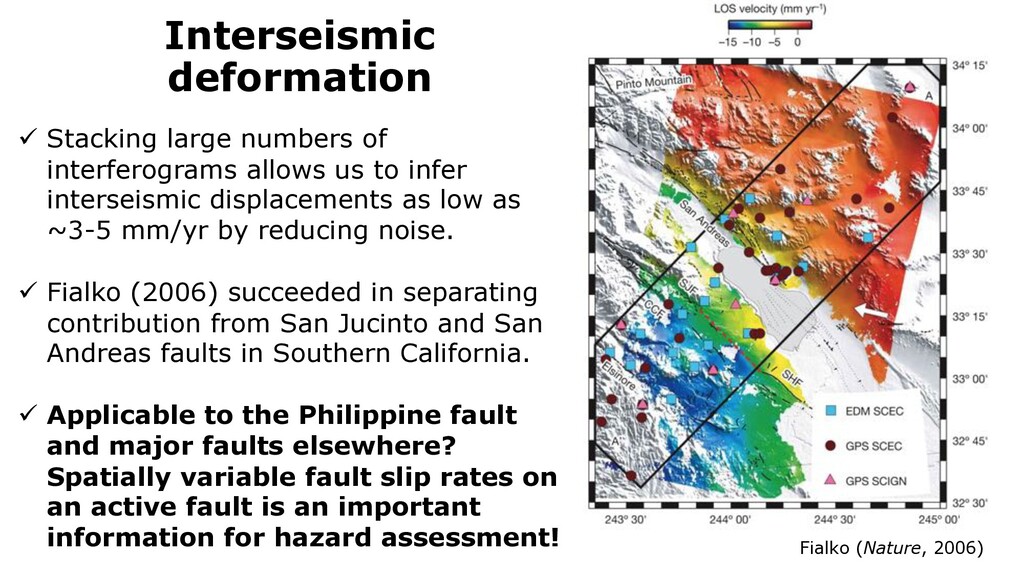
interferograms allows us to infer interseismic displacements as low as ~3-5 mm/yr by reducing noise. ü Fialko (2006) succeeded in separating contribution from San Jucinto and San Andreas faults in Southern California. ü Applicable to the Philippine fault and major faults elsewhere? Spatially variable fault slip rates on an active fault is an important information for hazard assessment!
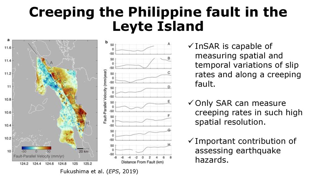
al. (EPS, 2019) ü InSAR is capable of measuring spatial and temporal variations of slip rates and along a creeping fault. ü Only SAR can measure creeping rates in such high spatial resolution. ü Important contribution of assessing earthquake hazards. Page 7 of 22 shima et al. Earth, Planets and Space (2019) 71:118 g. 6 a Mean velocity in the fault-parallel horizontal direction (N25◦ W). Direction N25◦ W is taken positive. b Velocity profiles along the lines own in a
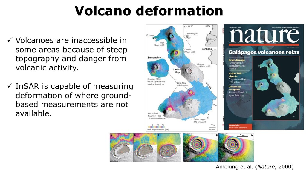
inaccessible in some areas because of steep topography and danger from volcanic activity. ü InSAR is capable of measuring deformation of where ground- based measurements are not available. With this background, SAR observations give us valuable informat tific interests as the study of Amelung et al. (2000) was on the cover o Figure 30: Cover of Nature on 26 October
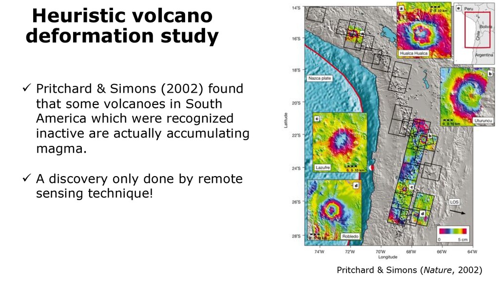
Pritchard & Simons (2002) found that some volcanoes in South America which were recognized inactive are actually accumulating magma. ü A discovery only done by remote sensing technique! Figure 32: An example of deformation in volcanoes which have been considered dormant.
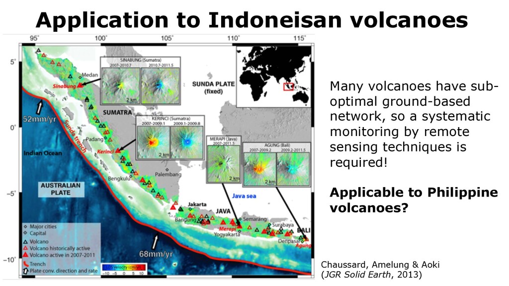
Earth, 2013) Many volcanoes have sub- optimal ground-based network, so a systematic monitoring by remote sensing techniques is required! Applicable to Philippine volcanoes?
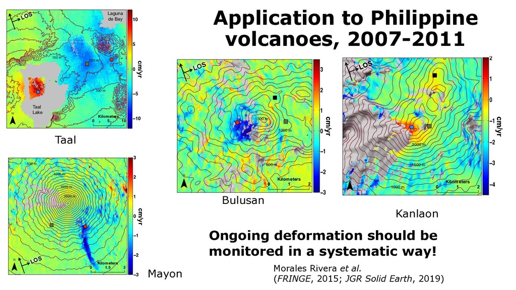
2015; JGR Solid Earth, 2019) various regions within the area (Fig. 2). 0 10 5 Kilometers ¯ 100 m 300 m 200 m 0 10 5 Kilometers ¯ 100 m 300 m 200 m ¯ 100 m 300 m 200 m 0 0.2 0.4 0.6 0.8 1 0 0.1 0.2 0.3 0.4 0.5 0.6 0.7 0.8 0.9 1 −10 −5 0 5 10 cm/yr Taal Lake LOS Laguna de Bay Kilometers 500 m 1000 m 1500 m 2000 m 0 3 1.5 Kilometers ¯ 500 m 1000 m 1500 m 2000 m ¯ 100 m 300 m 200 m 0 0.2 0.4 0.6 0.8 1 0 0.1 0.2 0.3 0.4 0.5 0.6 0.7 0.8 0.9 1 −3 −2 −1 0 1 2 3 cm/yr LOS it could possibly serve as evidence of the ctonic interactions within the region. The ould suggest that pressurization of the system led to inflation of the volcano, in stress transfers within the region and while the volcano continued to inflate. But ata and modeling is necessary to have an ding of the interactions occurring within the hich is out of the scope of this study. on olcano erupted lava flows during 2006 that placed in the SE flank of the volcano nian Institute, Global volcanism report, at http://www.volcano.si.edu). A LOS decrease is observed at Mayon volcano over osits, with a maximum rate of 3.5 cm/yr, likely d with cooling and compaction (Fig. 3). 3.3. Bulusan LOS velocity decrease is observed on the Western Flank of Bulusan volcano (Fig. 4), at a maximum rate of 3.5 cm/yr. The signal coincides with the end of the 2007 eruption phase, indicating possible depressurization of the volcanic system. 0 2 1 Kilometers ¯ 1500 m 1000 m 500 m 0 2 1 Kilometers ¯ 1500 m 1000 m 500 m 0 10 5 Kilometers ¯ 100 m 300 m 200 m cm/yr LOS 0 0.2 0.4 0.6 0.8 1 0 0.1 0.2 0.3 0.4 0.5 0.6 0.7 0.8 0.9 1 −3 −2 −1 0 1 2 3 Taal Mayon Bulusan Kanlaon deforming area is unknown due to the loss of coherence towards the W-SW flank of the volcano. The signal appears to be morphostructurally confined within a valley, and several scarp features can be observed with Google Earth imagery, suggesting that mass movements are the likely cause of the signal. 0 2 1 Kilometers ¯ 1500 m 2000 m 1000 m 0 2 1 Kilometers ¯ 1500 m 2000 m 1000 m 0 10 5 Kilometers ¯ 100 m 300 m 200 m cm/yr LOS 0 0.2 0.4 0.6 0.8 1 0 0.1 0.2 0.3 0.4 0.5 0.6 0.7 0.8 0.9 1 −4 −3 −2 −1 0 1 2 Ongoing deformation should be monitored in a systematic way!
vent: LOS velocity of about 38 mm/yr in the ALOS-1 period (2006-2011). Negligible deformation in the ALOS2 period (2014-2017). ü The 1977 vent: Maximum LOS velocities of about 66, 45 and 43 mm/yr in the JERS (1992-1998), ALOS-1 and ALOS-2 periods. ü The 1943 vent: Steady deformation with a maximum LOS velocity of about 20 mm/yr in 1992-2017. Ascending Descending 2000 1977 1943 Wang & Aoki (JGR Solid Earth, 2019)
between western ey are mostly between 1.5 and 2.5 years ation time is estimated only when an F-test (e.g., Menke, 2012, pp. 111–112) shows that an exponential curve fits the time series better than a linear fit with a confidence of 95%. Thus a relaxation time is not obtained from noisy or short time series. (Fig. 4). -7˚35 -7˚30 (a) 427-7030 a b c d LOS -7˚35 -7˚30 (b) 430-7020 a b c d LOS 112˚40 112˚45 -7˚35 -7˚30 (c) 91-3770 a b c d LOS 112˚40 -7˚35 -7˚30 (d) 92-3770 a b c d LOS 112˚45 5 km -100 -50 0 50 100 150 200 LOS displacement (mm) (e) 89-3780 2006 2008 2010 −300 −200 −100 0 100 200 300 427−7030 τ=2.52±0.34 yr 430−7020 89−3780 91−3770 τ=2.47±0.66 yr 92−3770 τ=2.09±0.03 yr (a) −7.5111°S 112.6583° E LOS change (mm) Year 2006 2008 2010 427−7030 τ=2.22±0.07 yr 430−7020 89−3780 91−3770 τ=1.35± 0.03 yr 92−3770 τ=1.83±0.03 yr (b) −7.5125°S 112.6778° E Year 2006 2008 2010 −300 −200 −100 0 100 200 300 427−7030 τ=2.93±0.47 yr 430−7020 89−3780 91−3770 92−3770 τ=1.63±0.02 yr (c) −7.5167°S 112.7000° E Year 2006 2008 2010 −300 −200 −100 0 100 200 300 427−7030 τ=2.21±0.24 yr 430−7020 89−3780 91−3770 τ=1.84±0.30 yr 92−3770 τ=1.64±0.15 yr (d) −7.5417°S 112.7000° E Year Fig. 4. Temporal evolution of LOS changes for four representative points whose location is shown in Fig. 3. Solid curves denote the calculated LOS changes by exponential curve fit the observed LOS changes more than two years after the onset of the eruption (t N 2008.408). They are shown only when an F-test (Menke, 2012, p. 111–112) gives a bett exponential fit than a straight-line regression by a confidence level of 95%. Y. Aoki, T.P. Sidiq / Journal of Volcanology and Geothermal Research 278–279 (2014) 96–102 Aoki & Sidiq (JVGR, 2014)
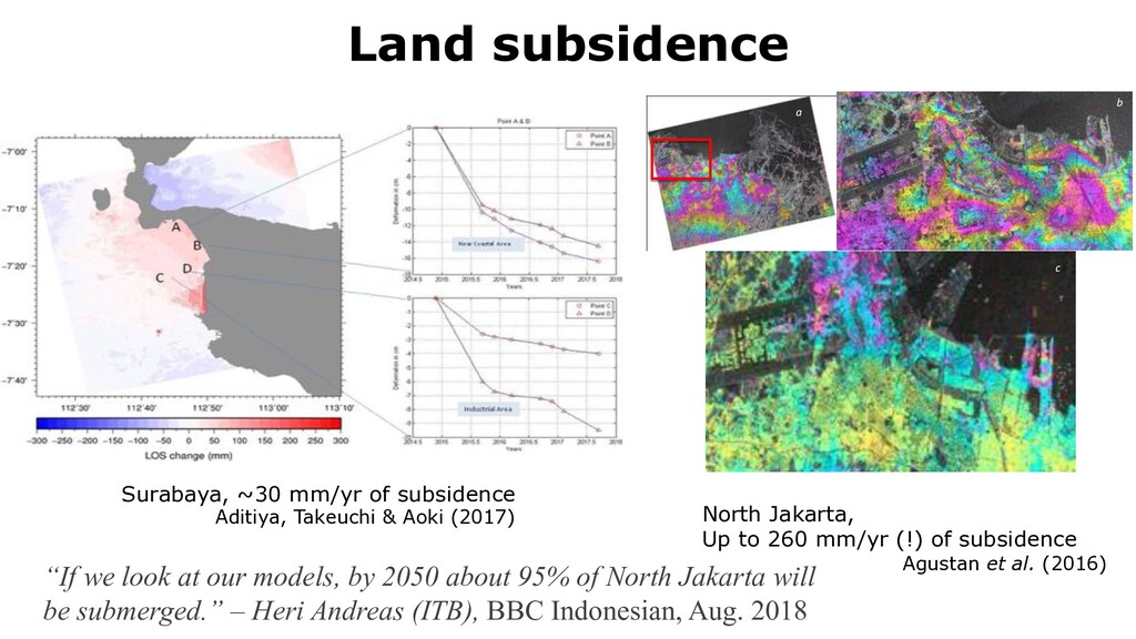
to 10 cm on points A and 6 cm on point D. r, in the northern part (Kenjeran sub-district) subsidence reach up to 2.2 cm/ year and the part is more lower reach up to 0.6 cm/ year. Generally the coherence value of ALOS-2 images than ALOS but the temporal resolution is opposite for the area in Indonesia. Figure 6. Plot of Specified Point in Surabaya lusions rk has presented an analysis of the ground subsidence phenomena in Surabaya City. The d multi-temporal InSAR technique is applied to this site using 8 ALOS-2 PALSAR-2 images from 2014 to 2017. We identified a few locations undergoing subsidence at rates up to 2,2 Figure 7. Identification of subsided areas in Jakarta based on DInSAR technique. (a) Interferogram from 2007-2011 based on ALOS-PALSAR data, (b) subsided area in Pluit region from 2007-2011 or 1472 days based on ALOS-PALSAR data, (c) subsided area in Pluit area from 2014 -2016 or 658 days based on ALOS-2 data, image not rectified. 4. Conclusions This research shows the ability of SAR data to identify ground deformation in Jakarta area by analysing the amplitude and phase components. Sentinel-1A data and S1TBX software are useful to obtain the land surface changes based on amplitude analysis. This research also found that atmospheric phase affects much to C-band SAR data as already identify by previous studies [11] and c b a Surabaya, ~30 mm/yr of subsidence Aditiya, Takeuchi & Aoki (2017) North Jakarta, Up to 260 mm/yr (!) of subsidence Agustan et al. (2016) “If we look at our models, by 2050 about 95% of North Jakarta will be submerged.” – Heri Andreas (ITB), BBC Indonesian, Aug. 2018
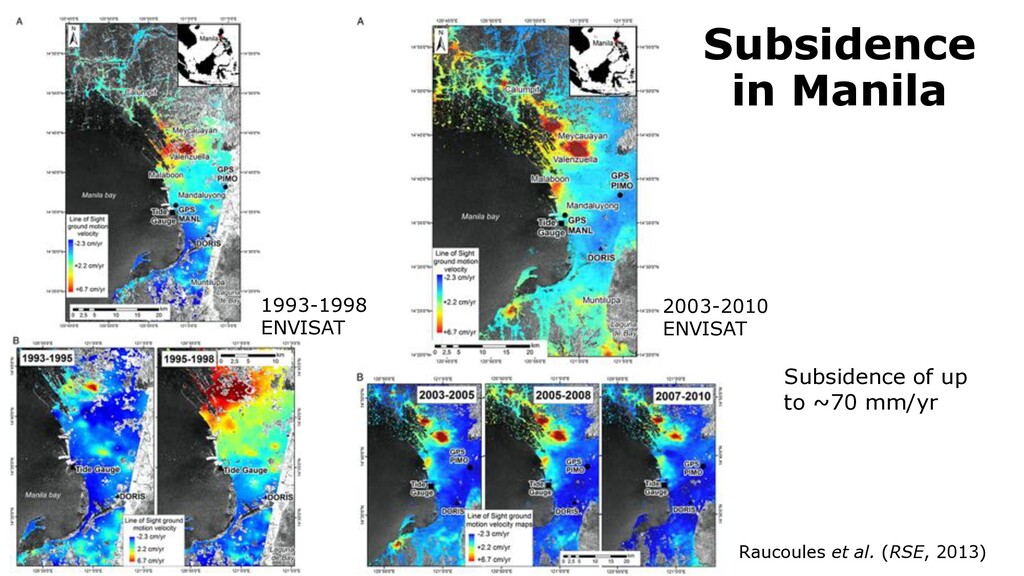
139 (2013) 386–397 Subsidence in Manila 389 D. Raucoules et al. / Remote Sensing of Environment 139 (2013) 386–397 1993-1998 ENVISAT 2003-2010 ENVISAT Raucoules et al. (RSE, 2013) Subsidence of up to ~70 mm/yr
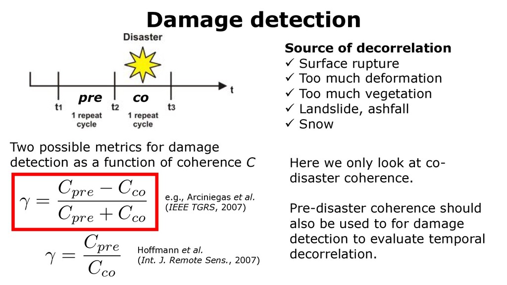
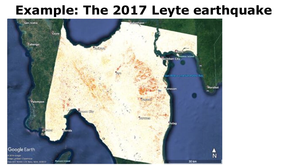
Cco mum case the temporal baseline between each acquisition is only one repeat so Section 4). (or more) SAR images, fulfilling the requirements mentioned above, are co-registered master image and resampled to its reference grid (Figure 4). Additionally, a common sures that only the overlapping parts of the spectrums are used. Thereby, the spatial fect (see Section 2.1.) is reduced [74]. In the next step, interferograms between he two slave images are generated: One pre-disaster InSAR pair (t1 and t2 ) and one R pair (t2 and t3 ). Then, for both InSAR pairs the coherence is computed according to e Section 2.1). Moreover, as described by Equation (9), also two SAR intensity computed using again the co-registered pre- (t1 and t2 ) and co-disaster (t2 and t3 ) airs [8]. The damage caused by the natural disaster is then assessed by detecting the he corresponding image pairs (see Section 2.3 for more details). pre co Two possible metrics for damage detection as a function of coherence C e.g., Arciniegas et al. (IEEE TGRS, 2007) Hoffmann et al. (Int. J. Remote Sens., 2007) Here we only look at co- disaster coherence. Pre-disaster coherence should also be used to for damage detection to evaluate temporal decorrelation. Source of decorrelation ü Surface rupture ü Too much deformation ü Too much vegetation ü Landslide, ashfall ü Snow
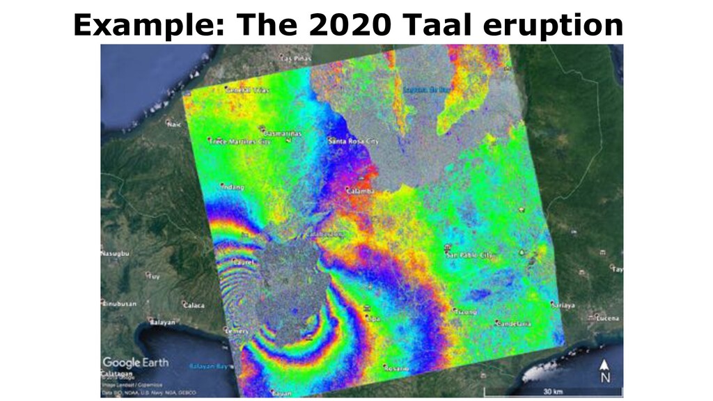
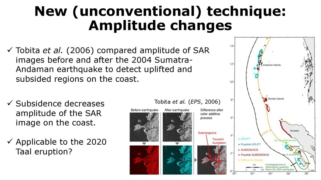
ü Tobita et al. (2006) compared amplitude of SAR images before and after the 2004 Sumatra- Andaman earthquake to detect uplifted and subsided regions on the coast. ü Subsidence decreases amplitude of the SAR image on the coast. ü Applicable to the 2020 Taal eruption?
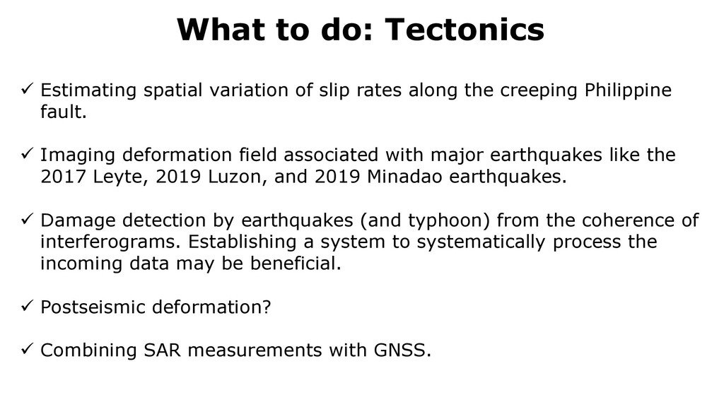
rates along the creeping Philippine fault. ü Imaging deformation field associated with major earthquakes like the 2017 Leyte, 2019 Luzon, and 2019 Minadao earthquakes. ü Damage detection by earthquakes (and typhoon) from the coherence of interferograms. Establishing a system to systematically process the incoming data may be beneficial. ü Postseismic deformation? ü Combining SAR measurements with GNSS.
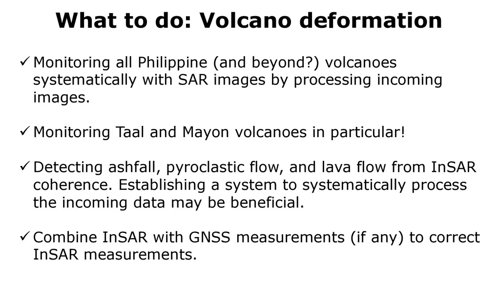
beyond?) volcanoes systematically with SAR images by processing incoming images. ü Monitoring Taal and Mayon volcanoes in particular! ü Detecting ashfall, pyroclastic flow, and lava flow from InSAR coherence. Establishing a system to systematically process the incoming data may be beneficial. ü Combine InSAR with GNSS measurements (if any) to correct InSAR measurements.
regardless of the weather. ü SAR can measure surface displacements associated with various phenomena with a spatial resolution, but with some limitations. ü SAR can be a powerful tool in detecting damages caused by landslide, flooding, tsunami, …. ü Philippine people will benefit a lot from SAR images!