Classification

Transcript

1. Classification Albert Bifet April 2012
2. COMP423A/COMP523A Data Stream Mining Outline 1. Introduction 2. Stream Algorithmics 3. Concept drift 4. Evaluation 5. Classification 6. Ensemble Methods 7. Regression 8. Clustering 9. Frequent Pattern Mining 10. Distributed Streaming
3. Data Streams Big Data & Real Time
4. Data stream classification cycle 1. Process an example at a time, and inspect it only once (at most) 2. Use a limited amount of memory 3. Work in a limited amount of time 4. Be ready to predict at any point
5. Classification Definition Given nC different classes, a classifier algorithm builds a model that predicts for every unlabelled instance I the class C to which it belongs with accuracy. Example A spam filter Example Twitter Sentiment analysis: analyze tweets with positive or negative feelings
6. Bayes Classifiers Na¨ ıve Bayes Based on Bayes Theorem: P(c|d) = P(c)P(d|c) P(d) posterior = prior × likelikood evidence Estimates the probability of observing attribute a and the prior probability P(c) Probability of class c given an instance d: P(c|d) = P(c) a∈d P(a|c) P(d)
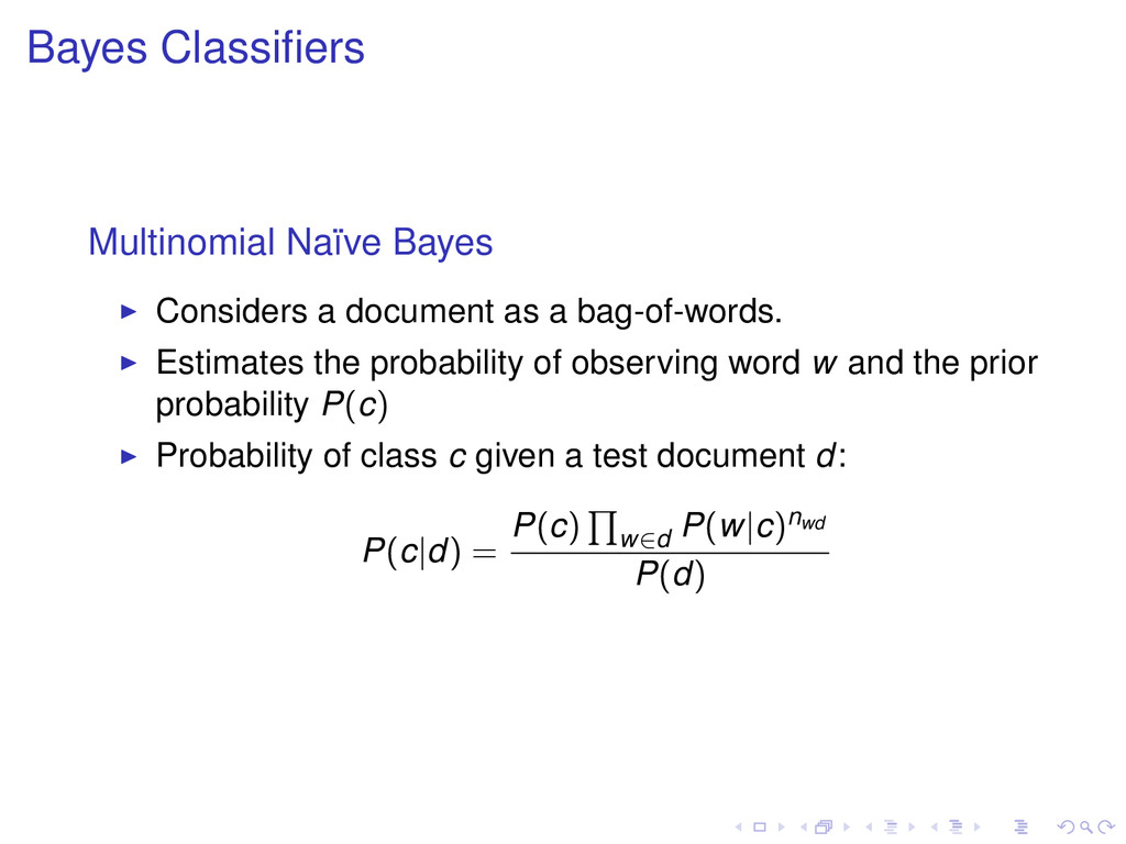
7. Bayes Classifiers Multinomial Na¨ ıve Bayes Considers a document as a bag-of-words. Estimates the probability of observing word w and the prior probability P(c) Probability of class c given a test document d: P(c|d) = P(c) w∈d P(w|c)nwd P(d)
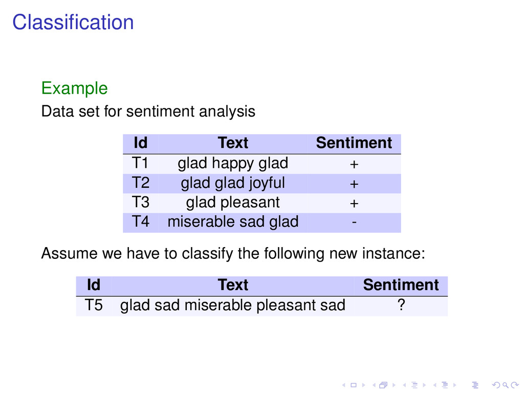
8. Classification Example Data set for sentiment analysis Id Text Sentiment T1 glad happy glad + T2 glad glad joyful + T3 glad pleasant + T4 miserable sad glad - Assume we have to classify the following new instance: Id Text Sentiment T5 glad sad miserable pleasant sad ?
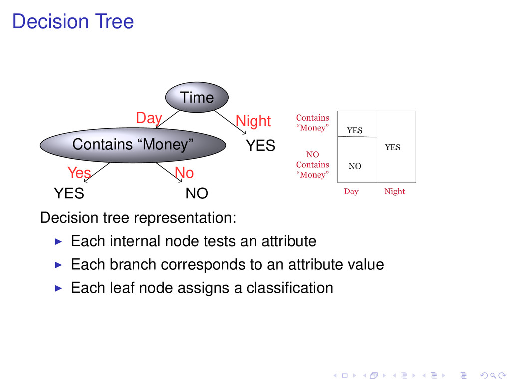
9. Decision Tree Time Contains “Money” YES Yes NO No Day YES Night Decision tree representation: Each internal node tests an attribute Each branch corresponds to an attribute value Each leaf node assigns a classification
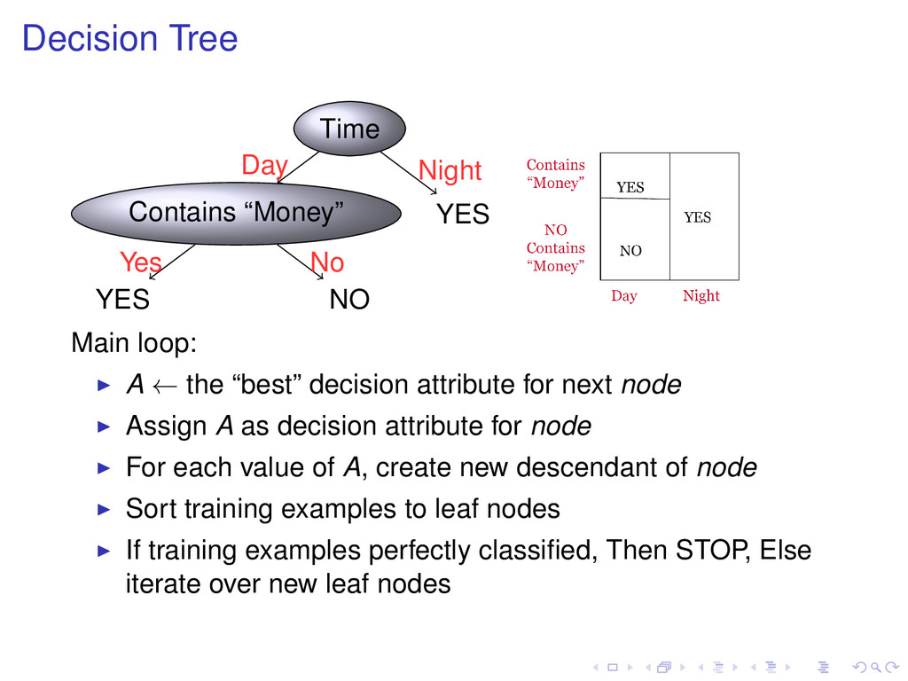
10. Decision Tree Time Contains “Money” YES Yes NO No Day YES Night Main loop: A ← the “best” decision attribute for next node Assign A as decision attribute for node For each value of A, create new descendant of node Sort training examples to leaf nodes If training examples perfectly classified, Then STOP, Else iterate over new leaf nodes
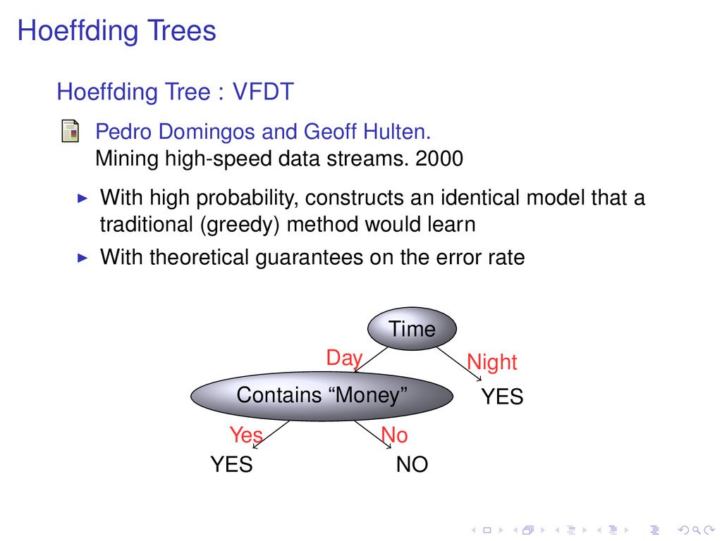
11. Hoeffding Trees Hoeffding Tree : VFDT Pedro Domingos and Geoff Hulten. Mining high-speed data streams. 2000 With high probability, constructs an identical model that a traditional (greedy) method would learn With theoretical guarantees on the error rate Time Contains “Money” YES Yes NO No Day YES Night
12. Hoeffding Bound Inequality Probability of deviation of its expected value.
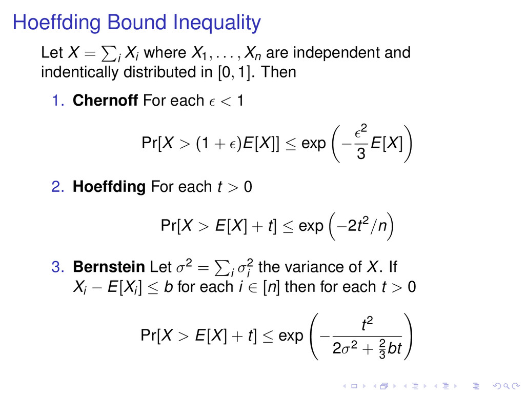
13. Hoeffding Bound Inequality Let X = i Xi where X1, . . . , Xn are independent and indentically distributed in [0, 1]. Then 1. Chernoff For each < 1 Pr[X > (1 + )E[X]] ≤ exp − 2 3 E[X] 2. Hoeffding For each t > 0 Pr[X > E[X] + t] ≤ exp −2t2/n 3. Bernstein Let σ2 = i σ2 i the variance of X. If Xi − E[Xi] ≤ b for each i ∈ [n] then for each t > 0 Pr[X > E[X] + t] ≤ exp − t2 2σ2 + 2 3 bt
14. Hoeffding Tree or VFDT HT(Stream, δ) 1 £ Let HT be a tree with a single leaf(root) 2 £ Init counts nijk at root 3 for each example (x, y) in Stream 4 do HTGROW((x, y), HT, δ)
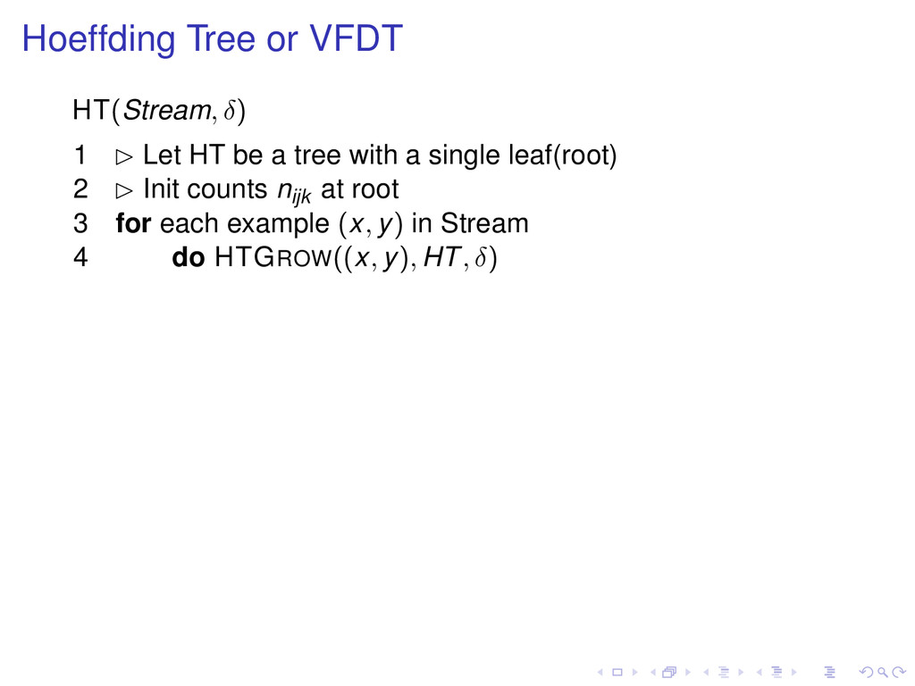
15. Hoeffding Tree or VFDT HT(Stream, δ) 1 £ Let HT be a tree with a single leaf(root) 2 £ Init counts nijk at root 3 for each example (x, y) in Stream 4 do HTGROW((x, y), HT, δ) HTGROW((x, y), HT, δ) 1 £ Sort (x, y) to leaf l using HT 2 £ Update counts nijk at leaf l 3 if examples seen so far at l are not all of the same class 4 then £ Compute G for each attribute 5 if G(Best Attr.)−G(2nd best) > R2 ln 1/δ 2n 6 then £ Split leaf on best attribute 7 for each branch 8 do £ Start new leaf and initiliatize counts
16. Hoeffding Trees HT features With high probability, constructs an identical model that a traditional (greedy) method would learn Ties: when two attributes have similar G, split if G(Best Attr.) − G(2nd best) < R2 ln 1/δ 2n < τ Compute G every nmin instances Memory: deactivate least promising nodes with lower pl × el pl is the probability to reach leaf l el is the error in the node
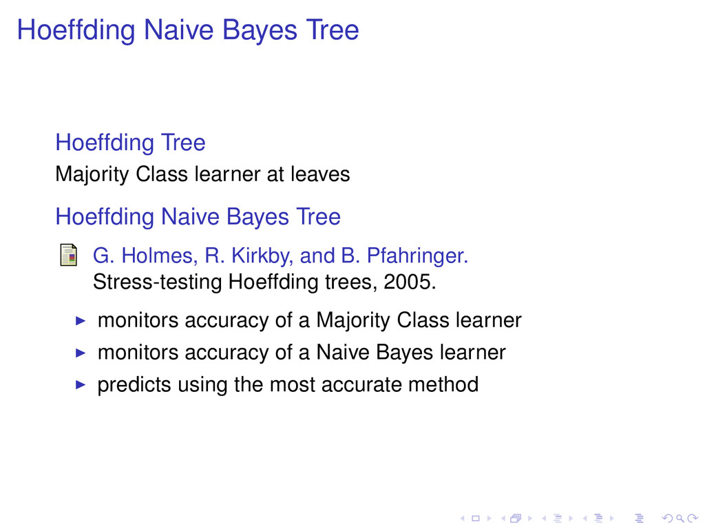
17. Hoeffding Naive Bayes Tree Hoeffding Tree Majority Class learner at leaves Hoeffding Naive Bayes Tree G. Holmes, R. Kirkby, and B. Pfahringer. Stress-testing Hoeffding trees, 2005. monitors accuracy of a Majority Class learner monitors accuracy of a Naive Bayes learner predicts using the most accurate method
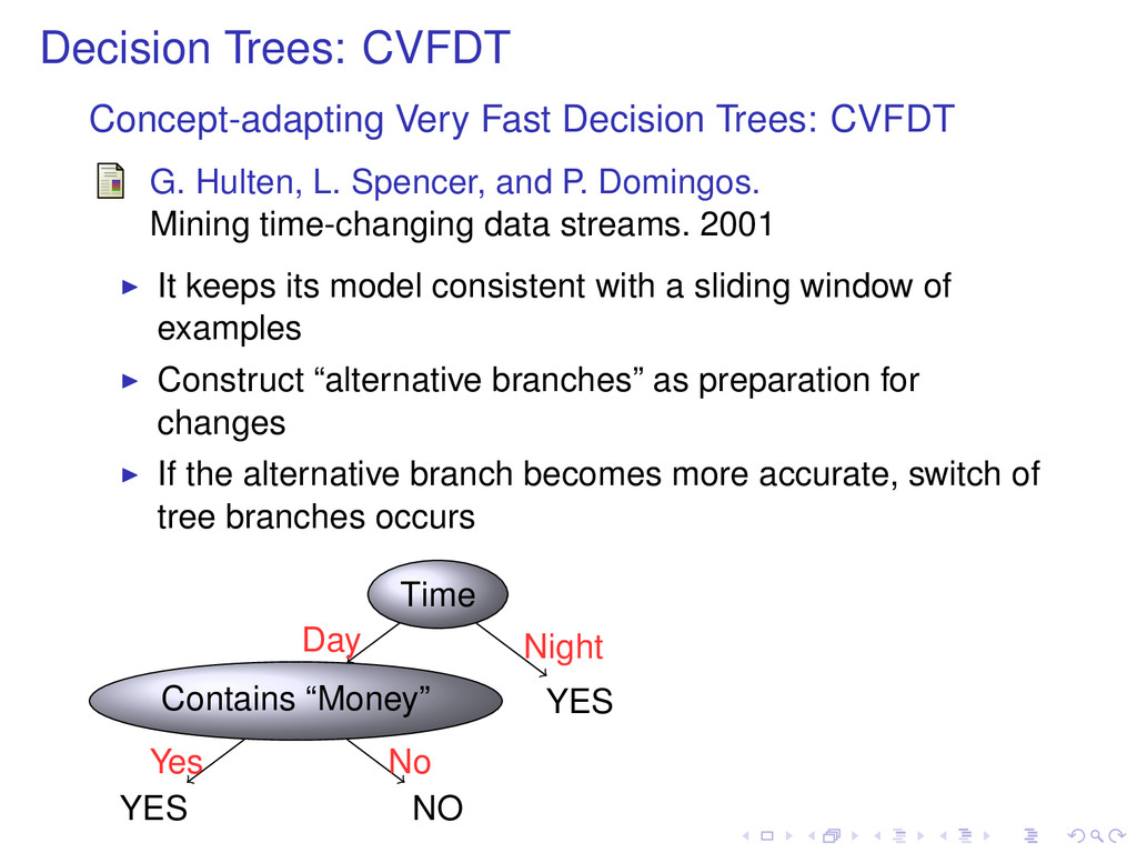
18. Decision Trees: CVFDT Concept-adapting Very Fast Decision Trees: CVFDT G. Hulten, L. Spencer, and P. Domingos. Mining time-changing data streams. 2001 It keeps its model consistent with a sliding window of examples Construct “alternative branches” as preparation for changes If the alternative branch becomes more accurate, switch of tree branches occurs Time Contains “Money” YES Yes NO No Day YES Night
19. Decision Trees: CVFDT Time Contains “Money” YES Yes NO No Day YES Night No theoretical guarantees on the error rate of CVFDT CVFDT parameters : 1. W: is the example window size. 2. T0: number of examples used to check at each node if the splitting attribute is still the best. 3. T1: number of examples used to build the alternate tree. 4. T2: number of examples used to test the accuracy of the alternate tree.
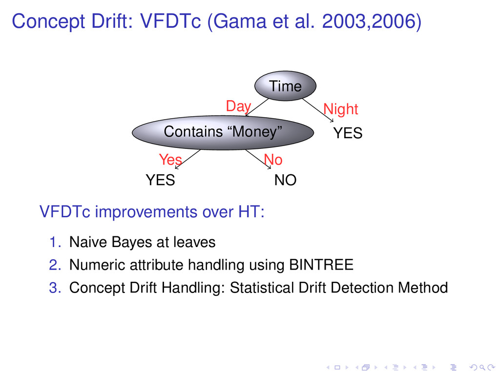
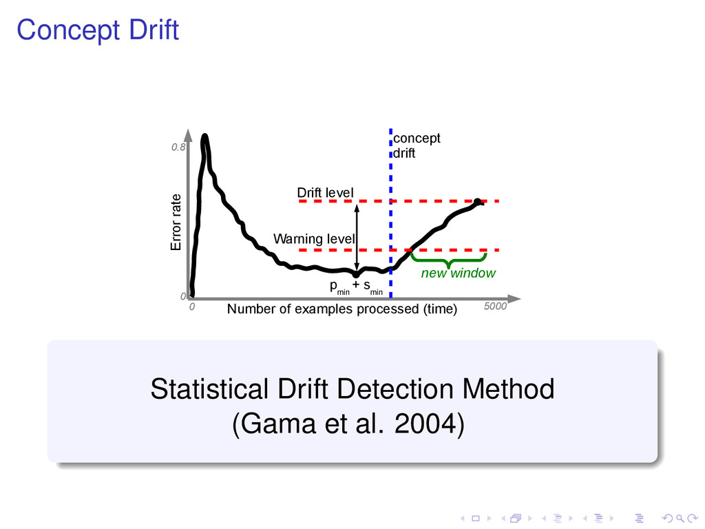
20. Concept Drift: VFDTc (Gama et al. 2003,2006) Time Contains “Money” YES Yes NO No Day YES Night VFDTc improvements over HT: 1. Naive Bayes at leaves 2. Numeric attribute handling using BINTREE 3. Concept Drift Handling: Statistical Drift Detection Method
21. Concept Drift Number of examples processed (time) Error rate concept drift p min + s min Drift level Warning level 0 5000 0 0.8 new window Statistical Drift Detection Method (Gama et al. 2004)
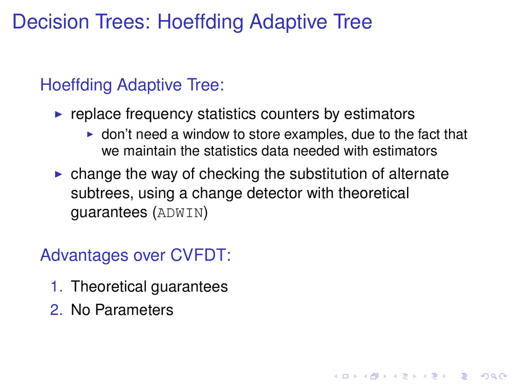
22. Decision Trees: Hoeffding Adaptive Tree Hoeffding Adaptive Tree: replace frequency statistics counters by estimators don’t need a window to store examples, due to the fact that we maintain the statistics data needed with estimators change the way of checking the substitution of alternate subtrees, using a change detector with theoretical guarantees (ADWIN) Advantages over CVFDT: 1. Theoretical guarantees 2. No Parameters
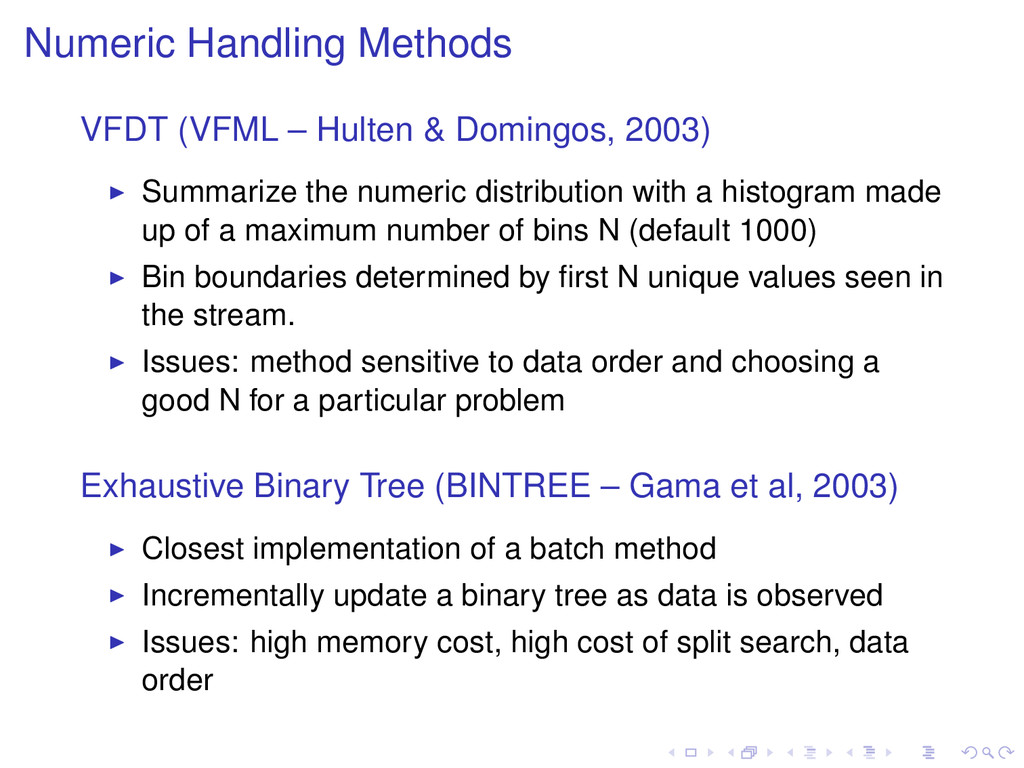
23. Numeric Handling Methods VFDT (VFML – Hulten & Domingos, 2003) Summarize the numeric distribution with a histogram made up of a maximum number of bins N (default 1000) Bin boundaries determined by first N unique values seen in the stream. Issues: method sensitive to data order and choosing a good N for a particular problem Exhaustive Binary Tree (BINTREE – Gama et al, 2003) Closest implementation of a batch method Incrementally update a binary tree as data is observed Issues: high memory cost, high cost of split search, data order
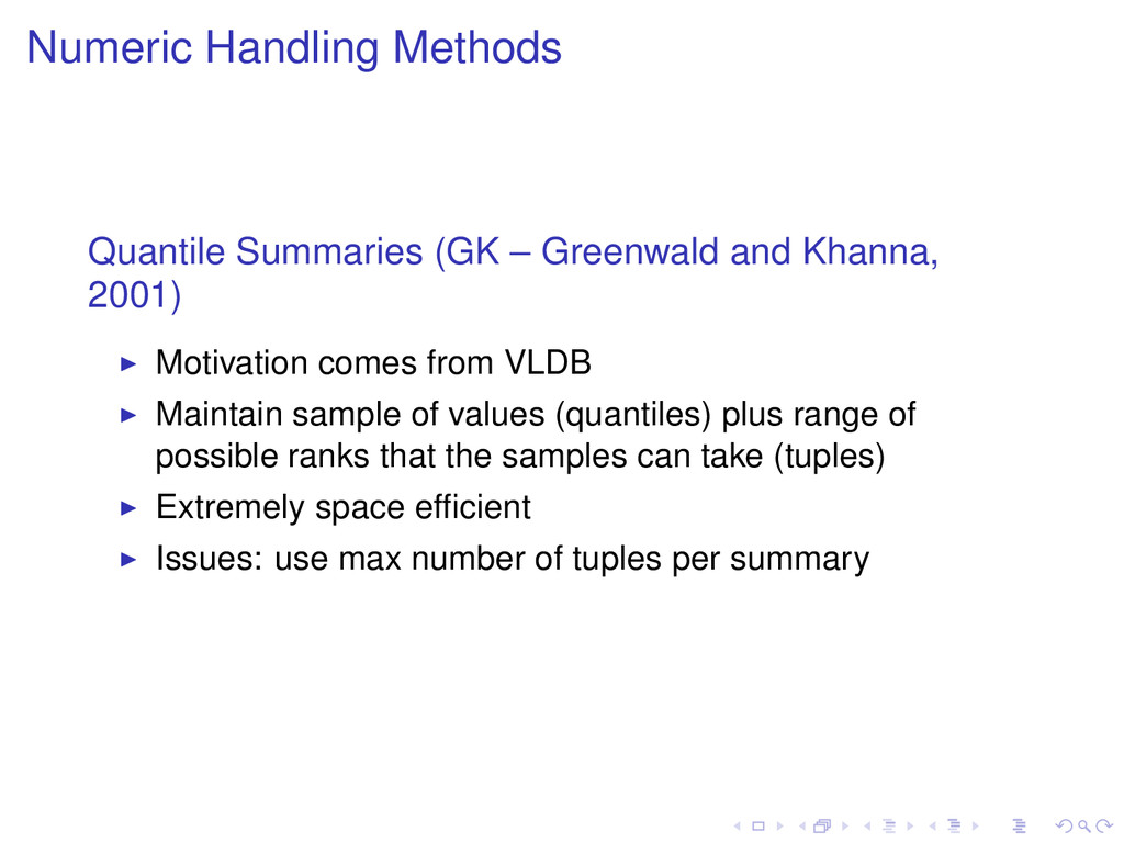
24. Numeric Handling Methods Quantile Summaries (GK – Greenwald and Khanna, 2001) Motivation comes from VLDB Maintain sample of values (quantiles) plus range of possible ranks that the samples can take (tuples) Extremely space efficient Issues: use max number of tuples per summary
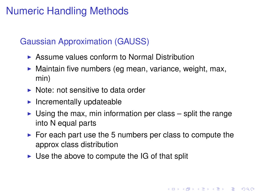
25. Numeric Handling Methods Gaussian Approximation (GAUSS) Assume values conform to Normal Distribution Maintain five numbers (eg mean, variance, weight, max, min) Note: not sensitive to data order Incrementally updateable Using the max, min information per class – split the range into N equal parts For each part use the 5 numbers per class to compute the approx class distribution Use the above to compute the IG of that split
26. Perceptron Attribute 1 Attribute 2 Attribute 3 Attribute 4 Attribute 5 Output hw (xi) w1 w2 w3 w4 w5 Data stream: xi, yi Classical perceptron: hw (xi) = sgn(wT xi), Minimize Mean-square error: J(w) = 1 2 (yi − hw (xi))2
27. Perceptron Attribute 1 Attribute 2 Attribute 3 Attribute 4 Attribute 5 Output hw (xi) w1 w2 w3 w4 w5 We use sigmoid function hw = σ(wT x) where σ(x) = 1/(1 + e−x ) σ (x) = σ(x)(1 − σ(x))
28. Perceptron Minimize Mean-square error: J(w) = 1 2 (yi − hw (xi))2 Stochastic Gradient Descent: w = w − η∇Jxi Gradient of the error function: ∇J = − i (yi − hw (xi))∇hw (xi) ∇hw (xi) = hw (xi)(1 − hw (xi)) Weight update rule w = w + η i (yi − hw (xi))hw (xi)(1 − hw (xi))xi
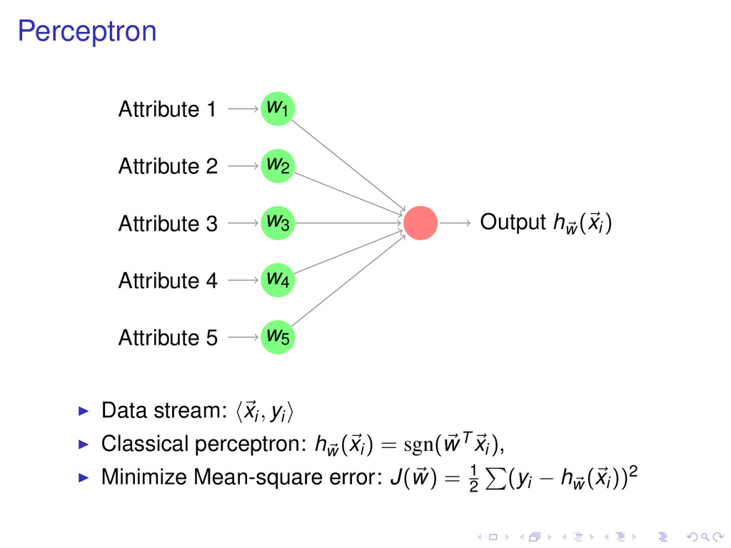
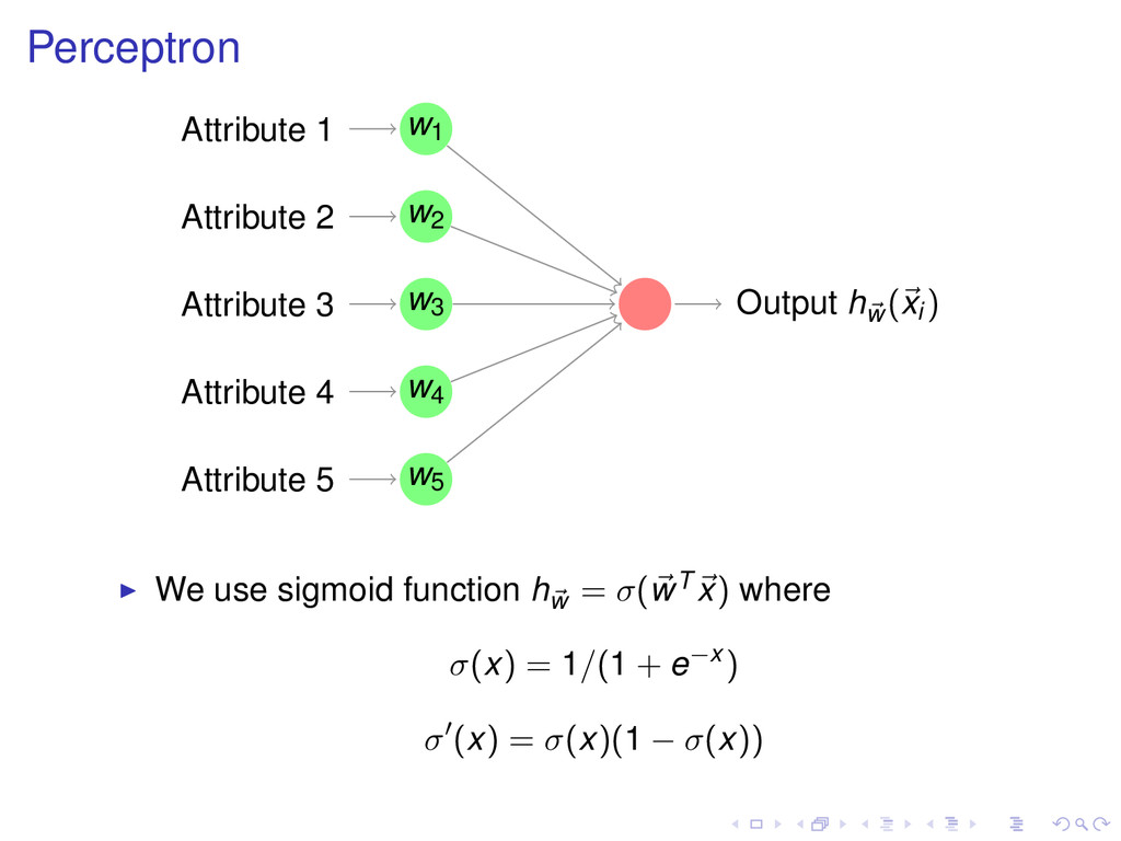
29. Perceptron PERCEPTRON LEARNING(Stream, η) 1 for each class 2 do PERCEPTRON LEARNING(Stream, class, η) PERCEPTRON LEARNING(Stream, class, η) 1 £ Let w0 and w be randomly initialized 2 for each example (x, y) in Stream 3 do if class = y 4 then δ = (1 − hw (x)) · hw (x) · (1 − hw (x)) 5 else δ = (0 − hw (x)) · hw (x) · (1 − hw (x)) 6 w = w + η · δ · x PERCEPTRON PREDICTION(x) 1 return arg maxclass hwclass (x)
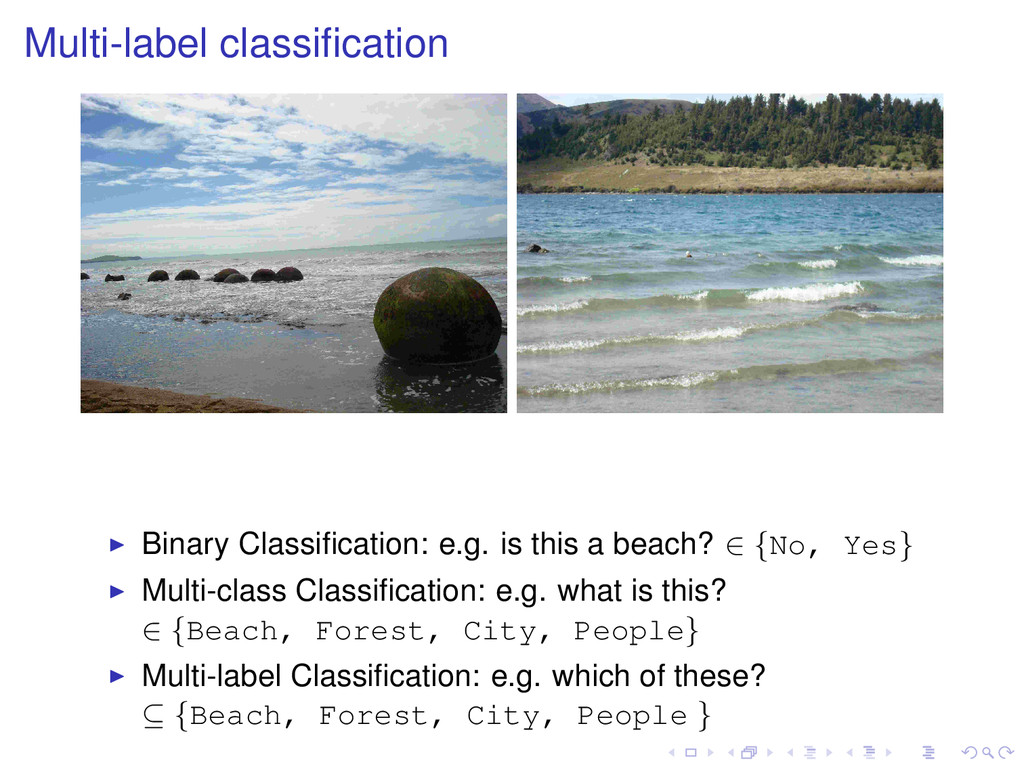
30. Multi-label classification Binary Classification: e.g. is this a beach? ∈ {No, Yes} Multi-class Classification: e.g. what is this? ∈ {Beach, Forest, City, People} Multi-label Classification: e.g. which of these? ⊆ {Beach, Forest, City, People }
31. Methods for Multi-label Classification Problem Transformation: Using off-the-shelf binary / multi-class classifiers for multi-label learning. Binary Relevance method (BR) One binary classifier for each label: simple; flexible; fast but does not explicitly model label dependencies Label Powerset method (LP) One multi-class classifier; one class for each labelset
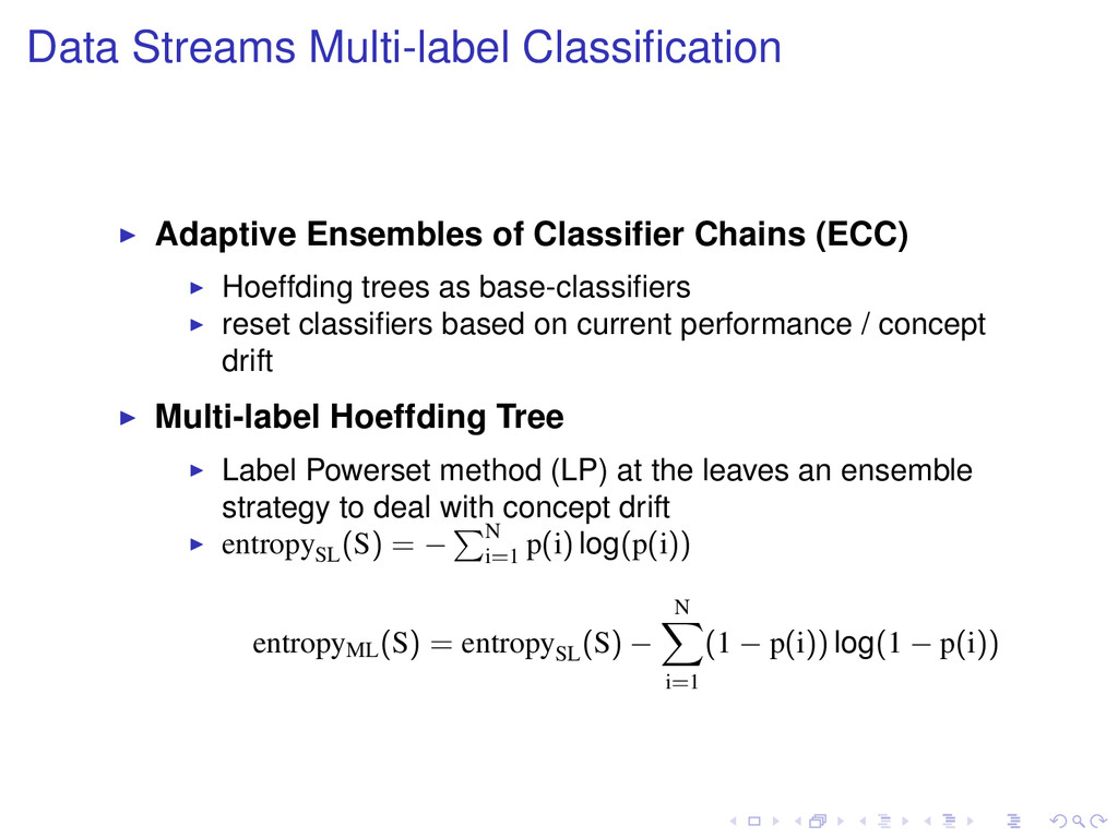
32. Data Streams Multi-label Classification Adaptive Ensembles of Classifier Chains (ECC) Hoeffding trees as base-classifiers reset classifiers based on current performance / concept drift Multi-label Hoeffding Tree Label Powerset method (LP) at the leaves an ensemble strategy to deal with concept drift entropySL (S) = − N i=1 p(i) log(p(i)) entropyML (S) = entropySL (S) − N i=1 (1 − p(i)) log(1 − p(i))
33. Active Learning ACTIVE LEARNING FRAMEWORK Input: labeling budget B and strategy parameters 1 for each Xt - incoming instance, 2 do if ACTIVE LEARNING STRATEGY(Xt , B, . . .) = true 3 then request the true label yt of instance Xt 4 train classifier L with (Xt , yt ) 5 if Ln exists then train classifier Ln with (Xt , yt ) 6 if change warning is signaled 7 then start a new classifier Ln 8 if change is detected 9 then replace classifier L with Ln
34. Active Learning Controlling Instance space Budget Coverage Random present full Fixed uncertainty no fragment Variable uncertainty handled fragment Randomized uncertainty handled full Table : Summary of strategies.