Concept Drift

Transcript

1. Concept Drift Albert Bifet March 2012
2. COMP423A/COMP523A Data Stream Mining Outline 1. Introduction 2. Stream Algorithmics 3. Concept drift 4. Evaluation 5. Classification 6. Ensemble Methods 7. Regression 8. Clustering 9. Frequent Pattern Mining 10. Distributed Streaming
3. Data Streams Big Data & Real Time
4. Data Mining Algorithms with Concept Drift. - input output DM Algorithm Static Model - Change Detect. - 6  - input output DM Algorithm - Estimator1 Estimator2 Estimator3 Estimator4 Estimator5
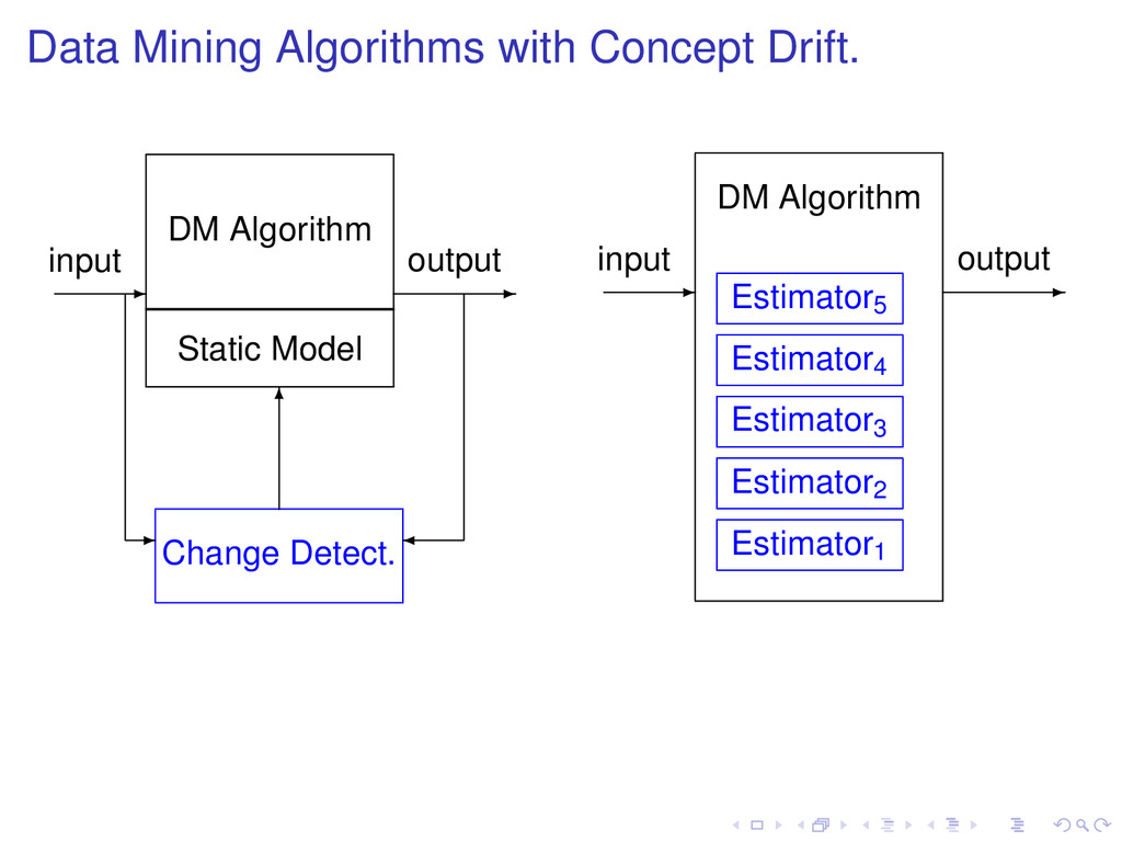
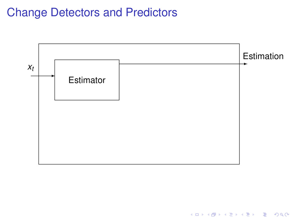
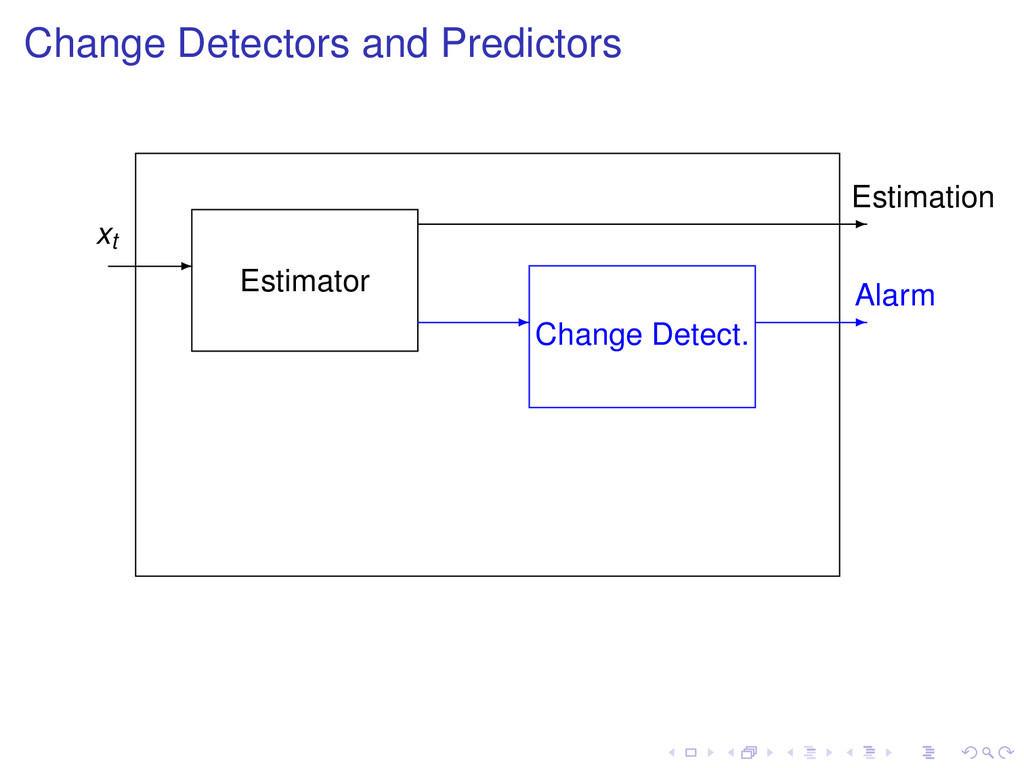
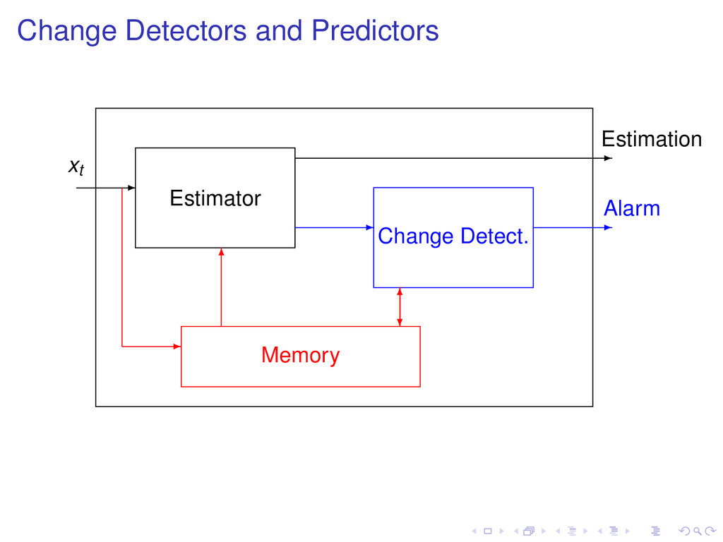
5. Introduction. Problem Given an input sequence x1, x2, · · · , xt we want to output at instant t an alarm signal if there is a distribution change and also a prediction xt+1 minimizing prediction error: |xt+1 − xt+1| Outputs an estimation of some important parameters of the input distribution, and a signal alarm indicating that distribution change has recently occurred.
6. Change Detectors and Predictors - xt Estimator - Estimation
7. Change Detectors and Predictors - xt Estimator - Estimation - - Alarm Change Detect.
8. Change Detectors and Predictors - xt Estimator - Estimation - - Alarm Change Detect. Memory - 6 6 ?
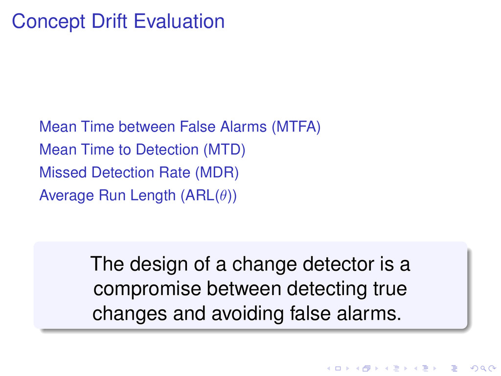
9. Concept Drift Evaluation Mean Time between False Alarms (MTFA) Mean Time to Detection (MTD) Missed Detection Rate (MDR) Average Run Length (ARL(θ)) The design of a change detector is a compromise between detecting true changes and avoiding false alarms.
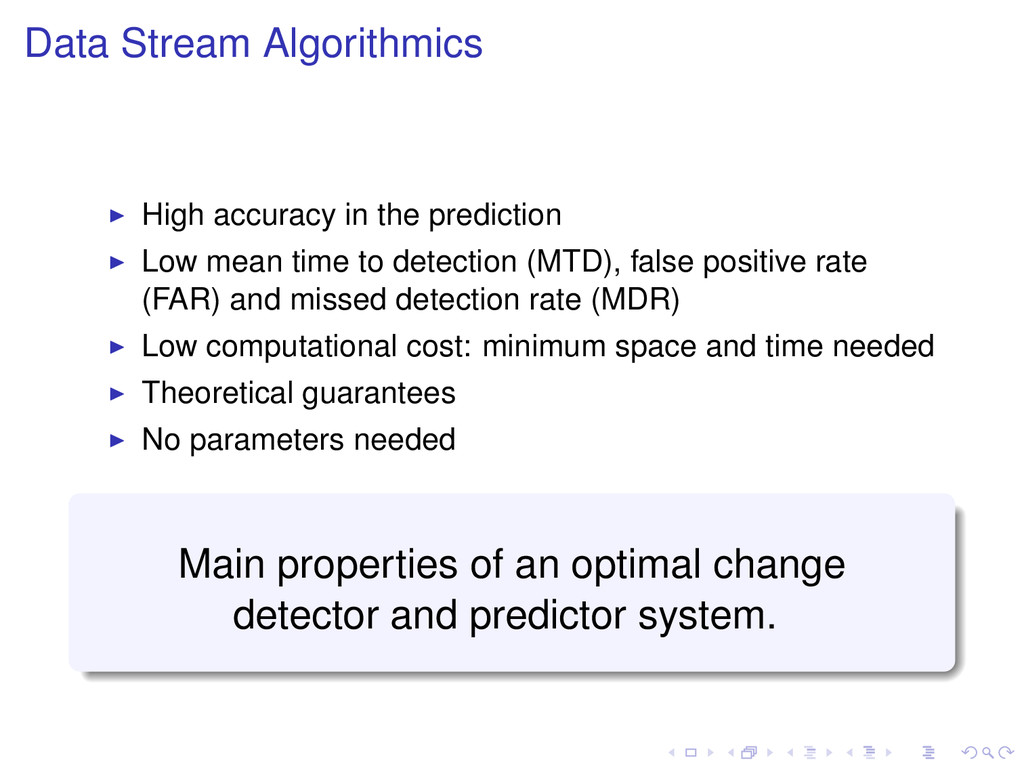
10. Data Stream Algorithmics High accuracy in the prediction Low mean time to detection (MTD), false positive rate (FAR) and missed detection rate (MDR) Low computational cost: minimum space and time needed Theoretical guarantees No parameters needed Main properties of an optimal change detector and predictor system.
11. The CUSUM Test The cumulative sum (CUSUM algorithm), gives an alarm when the mean of the input data is significantly different from zero. The CUSUM test is memoryless, and its accuracy depends on the choice of parameters υ and h. g0 = 0, gt = max (0, gt−1 + t − υ) if gt > h then alarm and gt = 0 Cumulative sum algorithm (CUSUM).
12. Page Hinckley Test The CUSUM test g0 = 0, gt = max (0, gt−1 + t − υ) if gt > h then alarm and gt = 0 The Page Hinckley Test g0 = 0, gt = gt−1 + ( t − υ) Gt = min(gt ) if gt − Gt > h then alarm and gt = 0
13. Geometric Moving Average Test The CUSUM test g0 = 0, gt = max (0, gt−1 + t − υ) if gt > h then alarm and gt = 0 The Geometric Moving Average Test g0 = 0, gt = λgt−1 + (1 − λ) t if gt > h then alarm and gt = 0 The forgetting factor λ is used to give more or less weight to the last data arrived.
14. Statistical test ˆ µ0 − ˆ µ1 ∈ N(0, σ2 0 + σ2 1 ), under H0 Example: Probability of false alarm of 5% Pr   |ˆ µ0 − ˆ µ1| σ2 0 + σ2 1 > h   = 0.05 As P(X < 1.96) = 0.975 the test becomes (ˆ µ0 − ˆ µ1)2 σ2 0 + σ2 1 > 1.962
15. Concept Drift 6 sigma
16. Concept Drift Number of examples processed (time) Error rate concept drift p min + s min Drift level Warning level 0 5000 0 0.8 new window Statistical Drift Detection Method (Joao Gama et al. 2004)
17. ADWIN: Adaptive Data Stream Sliding Window Let W = 101010110111111 Equal & fixed size subwindows: 1010 1011011 1111 Equal size adjacent subwindows: 1010101 1011 1111 Total window against subwindow: 10101011011 1111 ADWIN: All adjacent subwindows: 1 01010110111111 1010 10110111111 1010101 10111111 1010101101 11111 10101011011111 1
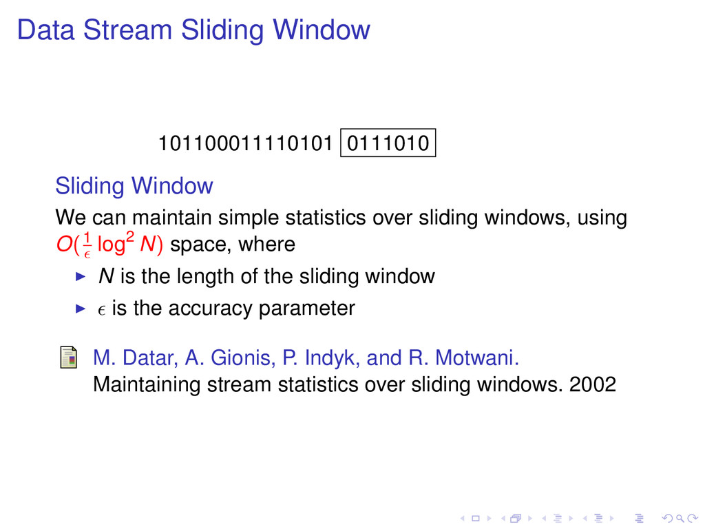
18. Data Stream Sliding Window 101100011110101 0111010 Sliding Window We can maintain simple statistics over sliding windows, using O(1 log2 N) space, where N is the length of the sliding window is the accuracy parameter M. Datar, A. Gionis, P. Indyk, and R. Motwani. Maintaining stream statistics over sliding windows. 2002
19. Exponential Histograms M = 2 1010101 101 11 1 1 1 Content: 4 2 2 1 1 1 Capacity: 7 3 2 1 1 1 1010101 101 11 11 1 Content: 4 2 2 2 1 Capacity: 7 3 2 2 1 1010101 10111 11 1 Content: 4 4 2 1 Capacity: 7 5 2 1
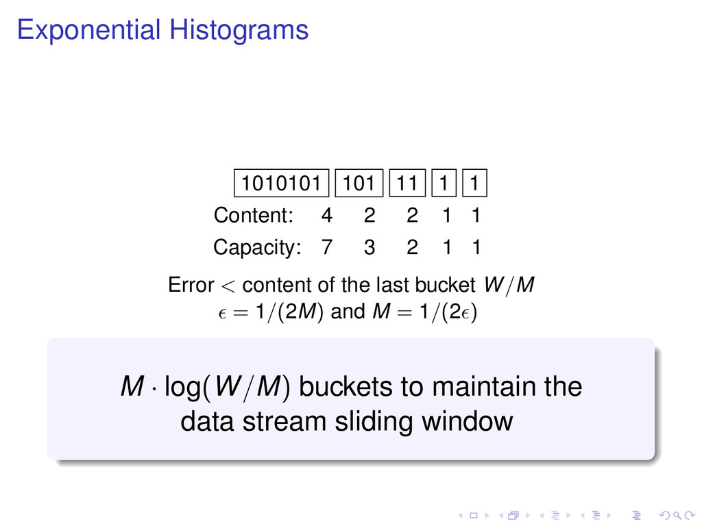
20. Exponential Histograms 1010101 101 11 1 1 Content: 4 2 2 1 1 Capacity: 7 3 2 1 1 Error < content of the last bucket W/M = 1/(2M) and M = 1/(2 ) M · log(W/M) buckets to maintain the data stream sliding window
21. Exponential Histograms 1010101 101 11 1 1 Content: 4 2 2 1 1 Capacity: 7 3 2 1 1 To give answers in O(1) time, it maintain three counters LAST, TOTAL and VARIANCE. M · log(W/M) buckets to maintain the data stream sliding window
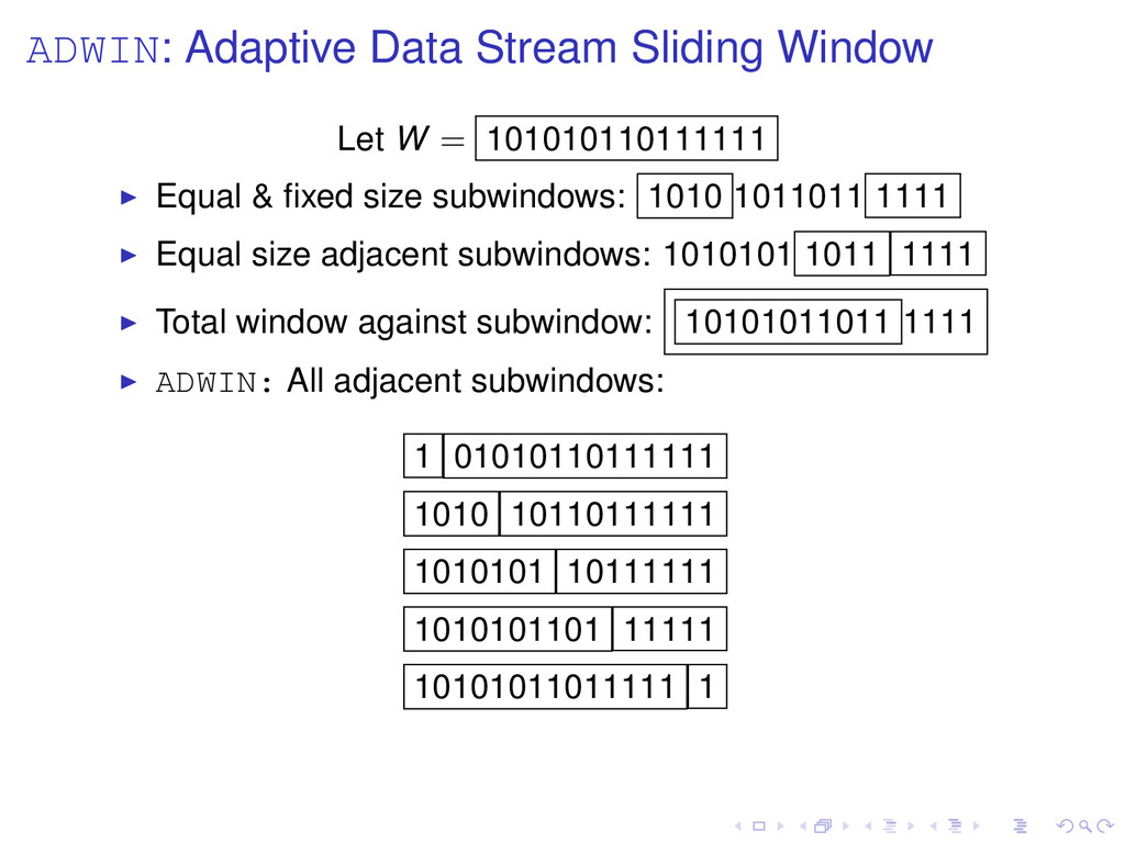
22. Algorithm ADaptive Sliding WINdow ADWIN: ADAPTIVE WINDOWING ALGORITHM 1 Initialize W as an empty list of buckets 2 Initialize WIDTH, VARIANCE and TOTAL 3 for each t > 0 4 do SETINPUT(xt , W) 5 output ˆ µW as TOTAL/WIDTH and ChangeAlarm SETINPUT(item e, List W) 1 INSERTELEMENT(e, W) 2 repeat DELETEELEMENT(W) 3 until |ˆ µW0 − ˆ µW1 | < cut holds 4 for every split of W into W = W0 · W1
23. Algorithm ADaptive Sliding WINdow INSERTELEMENT(item e, List W) 1 create a new bucket b with content e and capacity 1 2 W ← W ∪ {b} (i.e., add e to the head of W) 3 update WIDTH, VARIANCE and TOTAL 4 COMPRESSBUCKETS(W) DELETEELEMENT(List W) 1 remove a bucket from tail of List W 2 update WIDTH, VARIANCE and TOTAL 3 ChangeAlarm ← true
24. Algorithm ADaptive Sliding WINdow COMPRESSBUCKETS(List W) 1 Traverse the list of buckets in increasing order 2 do If there are more than M buckets of the same capacity 3 do merge buckets 4 COMPRESSBUCKETS(sublist of W not traversed)
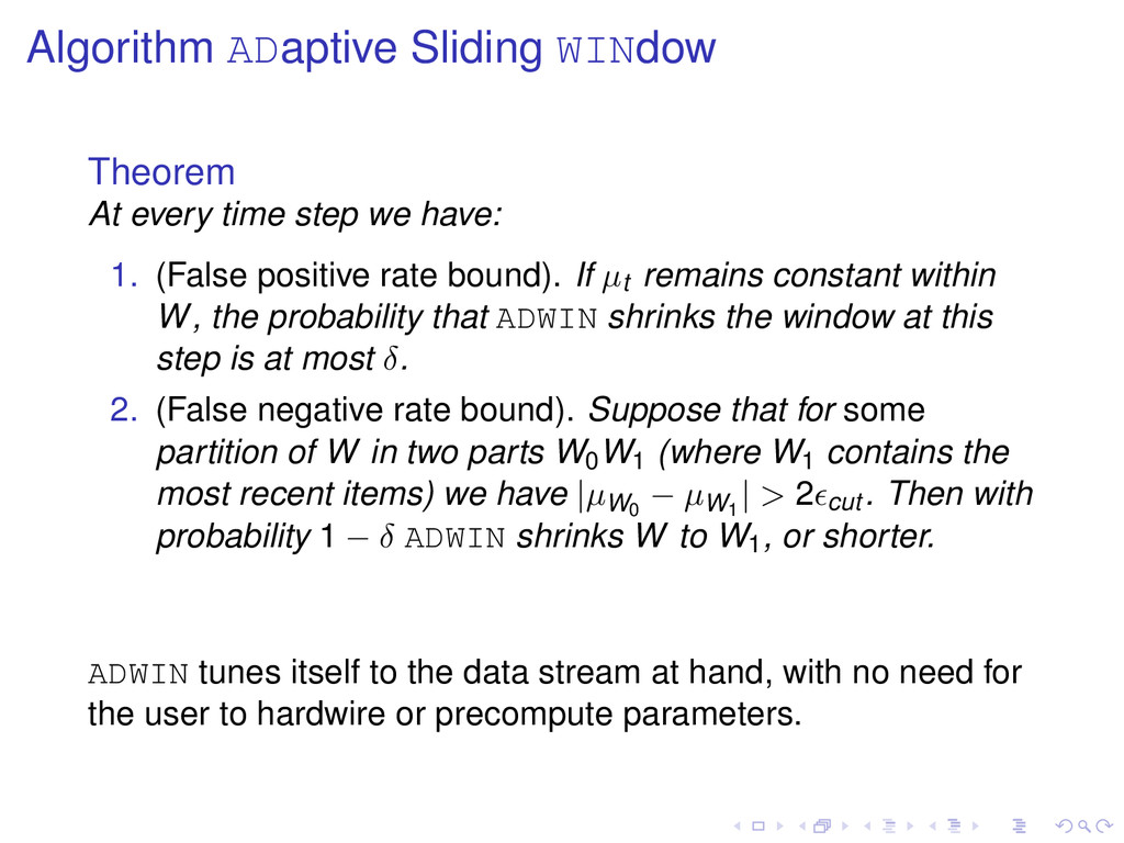
25. Algorithm ADaptive Sliding WINdow Theorem At every time step we have: 1. (False positive rate bound). If µt remains constant within W, the probability that ADWIN shrinks the window at this step is at most δ. 2. (False negative rate bound). Suppose that for some partition of W in two parts W0W1 (where W1 contains the most recent items) we have |µW0 − µW1 | > 2 cut . Then with probability 1 − δ ADWIN shrinks W to W1, or shorter. ADWIN tunes itself to the data stream at hand, with no need for the user to hardwire or precompute parameters.
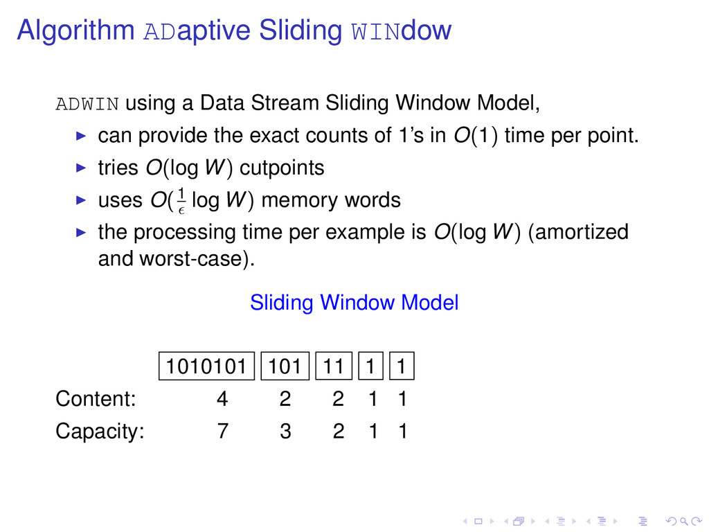
26. Algorithm ADaptive Sliding WINdow ADWIN using a Data Stream Sliding Window Model, can provide the exact counts of 1’s in O(1) time per point. tries O(log W) cutpoints uses O(1 log W) memory words the processing time per example is O(log W) (amortized and worst-case). Sliding Window Model 1010101 101 11 1 1 Content: 4 2 2 1 1 Capacity: 7 3 2 1 1