Regression

Transcript

1. Regression Albert Bifet May 2012
2. COMP423A/COMP523A Data Stream Mining Outline 1. Introduction 2. Stream Algorithmics 3. Concept drift 4. Evaluation 5. Classification 6. Ensemble Methods 7. Regression 8. Clustering 9. Frequent Pattern Mining 10. Distributed Streaming
3. Data Streams Big Data & Real Time
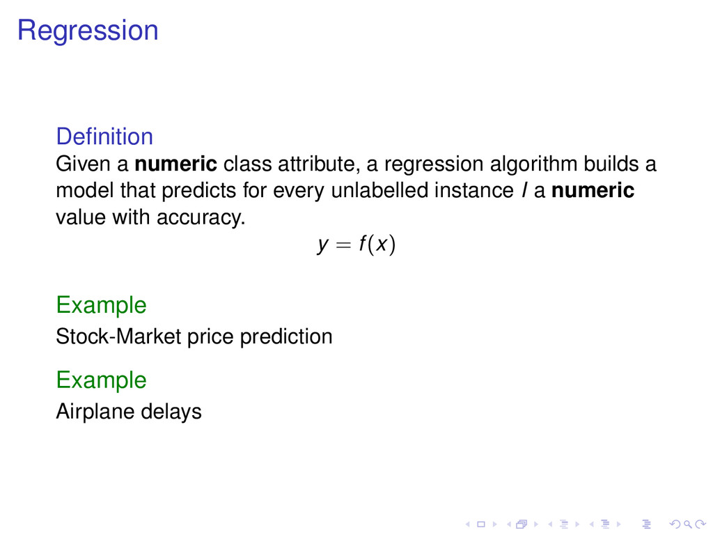
4. Regression Definition Given a numeric class attribute, a regression algorithm builds a model that predicts for every unlabelled instance I a numeric value with accuracy. y = f(x) Example Stock-Market price prediction Example Airplane delays
5. Evaluation 1. Error estimation: Hold-out or Prequential 2. Evaluation performance measures: MSE or MAE 3. Statistical significance validation: Nemenyi test Evaluation Framework
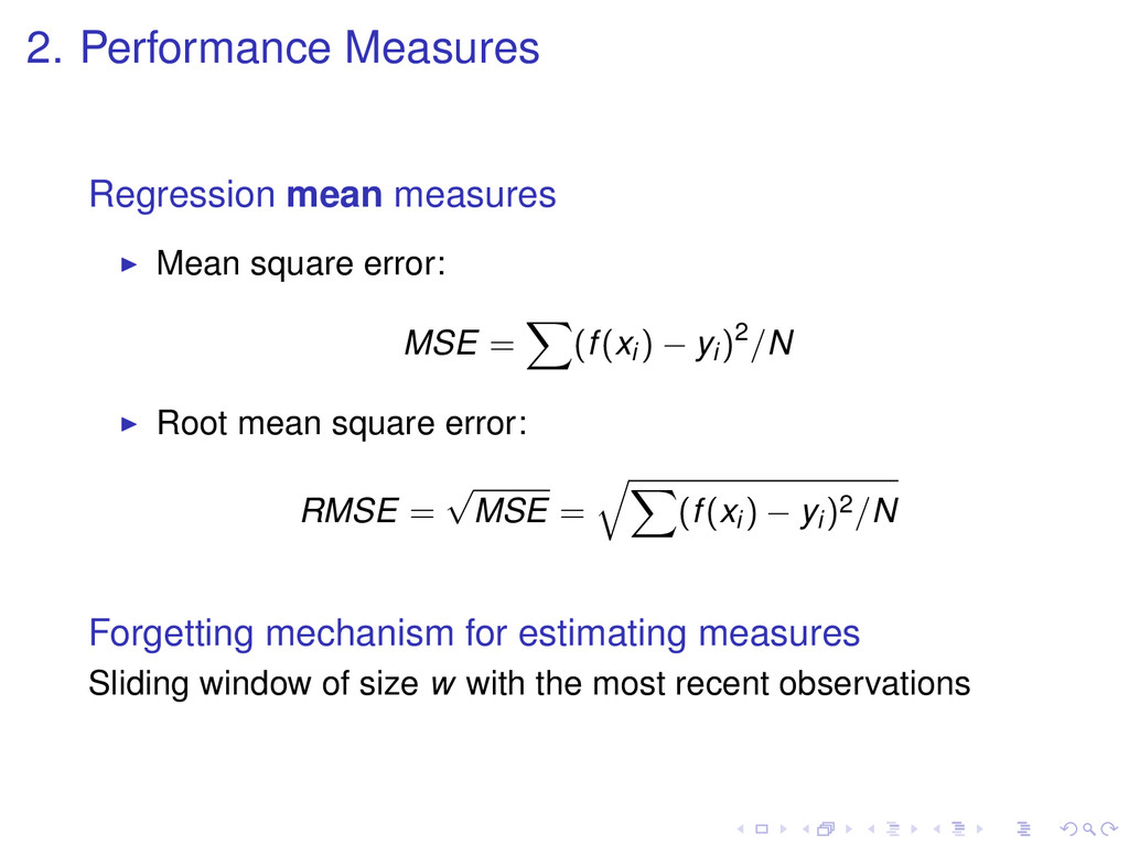
6. 2. Performance Measures Regression mean measures Mean square error: MSE = (f(xi) − yi)2/N Root mean square error: RMSE = √ MSE = (f(xi) − yi)2/N Forgetting mechanism for estimating measures Sliding window of size w with the most recent observations
7. 2. Performance Measures Regression relative measures Relative Square error: RSE = (f(xi) − yi)2/ (¯ yi − yi)2 Root relative square error: RRSE = √ RSE = (f(xi) − yi)2/ (¯ yi) − yi)2 Forgetting mechanism for estimating measures Sliding window of size w with the most recent observations
8. 2. Performance Measures Regression absolute measures Mean absolute error: MAE = (|f(xi) − yi|)/N Relative absolute error: RAE = (|f(xi) − yi|)/ (|ˆ yi − yi|) Forgetting mechanism for estimating measures Sliding window of size w with the most recent observations
9. Linear Methods for Regression Linear Least Squares fitting Linear Regression Model f(x) = β0 + p j=1 βj xj = Xβ Minimize residual sum of squares RSS(β) = N i=1 (yi − f(xi))2/N = (y − Xβ) (y − Xβ) Solution: ˆ β = (X X)−1X y
10. Perceptron Attribute 1 Attribute 2 Attribute 3 Attribute 4 Attribute 5 Output hw (xi) w1 w2 w3 w4 w5 Data stream: xi, yi Classical perceptron: hw (xi) = wT xi , Minimize Mean-square error: J(w) = 1 2 (yi − hw (xi))2
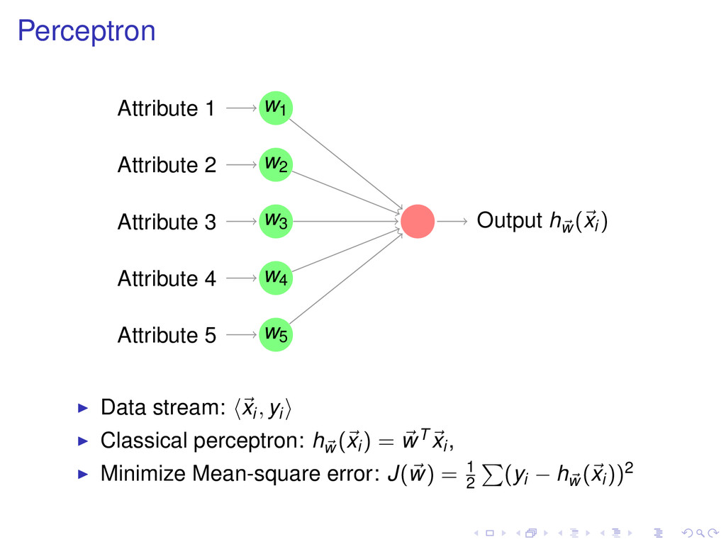
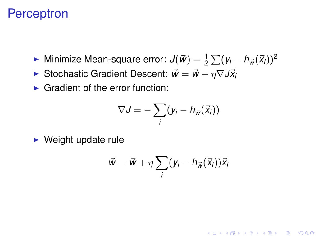
11. Perceptron Minimize Mean-square error: J(w) = 1 2 (yi − hw (xi))2 Stochastic Gradient Descent: w = w − η∇Jxi Gradient of the error function: ∇J = − i (yi − hw (xi)) Weight update rule w = w + η i (yi − hw (xi))xi
12. Fast Incremental Model Tree with Drift Detection FIMT-DD FIMT-DD differences with HT: 1. Splitting Criterion 2. Numeric attribute handling using BINTREE 3. Linear model at the leaves 4. Concept Drift Handling: Page-Hinckley 5. Alternate Tree adaption strategy
13. Splitting Criterion Standard Deviation Reduction Measure Classification Information Gain = Entropy(before Split) − Entropy(after split) Entropy = − c pi · log pi Gini Index = c pi(1 − pi) = 1 − c p2 i Regression Gain = SD(before Split) − SD(after split) StandardDeviation (SD) = (¯ y − yi)2/N
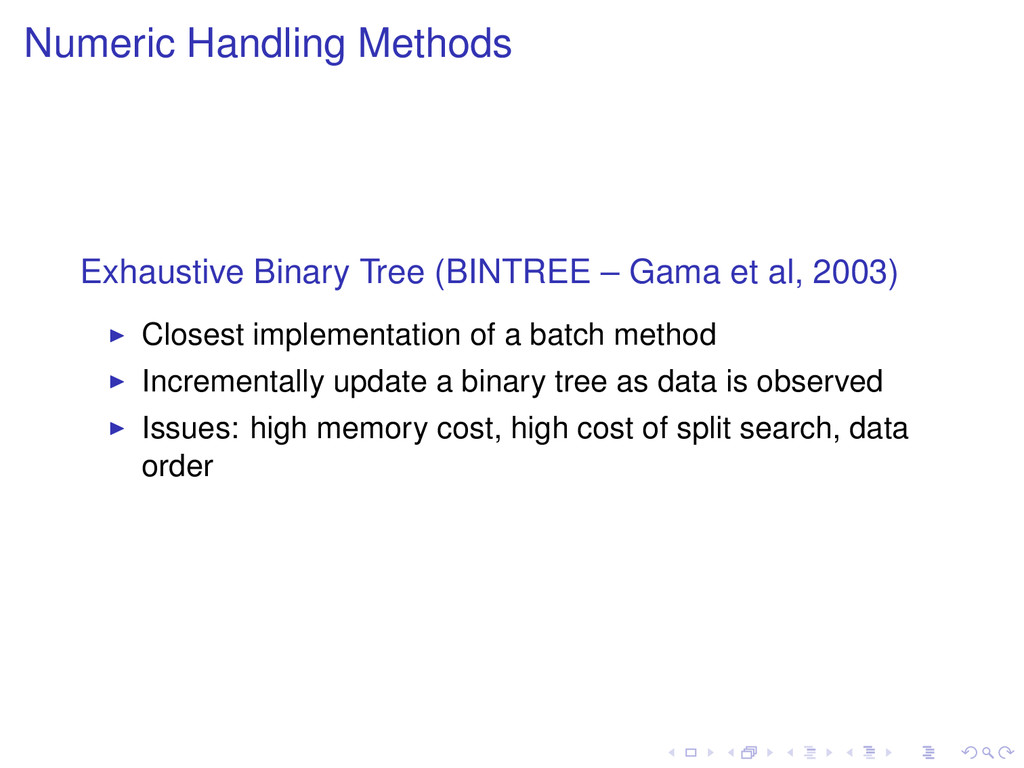
14. Numeric Handling Methods Exhaustive Binary Tree (BINTREE – Gama et al, 2003) Closest implementation of a batch method Incrementally update a binary tree as data is observed Issues: high memory cost, high cost of split search, data order
15. Page Hinckley Test The CUSUM test g0 = 0, gt = max (0, gt−1 + t − υ) if gt > h then alarm and gt = 0 The Page Hinckley Test g0 = 0, gt = gt−1 + ( t − υ) Gt = min(gt ) if gt − Gt > h then alarm and gt = 0
16. Lazy Methods kNN Nearest Neighbours: 1. Mean value of the k nearest neighbours ˆ f(xq) = k i=1 f(xi) k 2. Depends on distance function