Deep Learning in Scala 3 from scratch

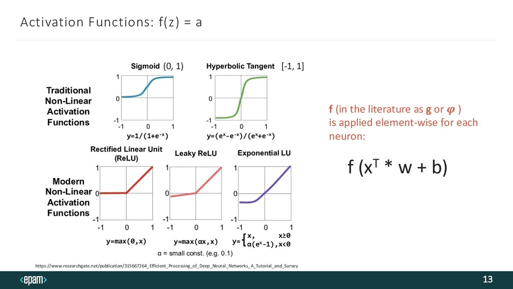
Scala as language with it's ability to write highly concise and declarative code, is a perfect match to express neural network algorithms as well. We will leverage features like type inference, the REPL, operator overloading, extension
methods, first class functions as well as the new Scala 3 "optional
braces syntax" to implement Deep Learning Algorithms.

Transcript

1. Deep Learning in
   Scala 3
   from scratch
   Alexey Novakov
   Rhein-Main Scala Enthusiasts
   

   View Slide

2. About Me
   • Solution Architect at EPAM Germany (BigData,
   Cloud)
   • Functional Programmer
   • 5 years working with Scala, 10 years with Java
   • I often talk at Rhein-Main Scala Enthusiasts
   Meetup
   • I like music, guitars and astronomy
   ALEXEY NOVAKOV
   2
   Twitter: @alexey_novakov
   Blog: https://novakov-alexey.github.io/
   

   View Slide

3. Goal of the Talk
   • Get an idea of the Deep Neural Network computation
   • Use Scala 3 features in the implementation
   • Inspire someone to write good & long-lasting Scala library
   for Deep Learning
   

   View Slide

4. Agenda
   #
   #
   #
   #
   #
   I N T R O T O D E E P L E A R N I N G
   T E N S O R S
   N E T W O R K I M P L E M E N T A T I O N
   M O D E L T R A I N I N G , T E S T
   M E T R I C S V I S U A L I Z A T I O N
   4
   

   View Slide

5. INTRO TO DEEP LEARNING
   5
   

   View Slide

6. Neuron Model
   6
   Biological nueron model
   !𝑥𝑖
   𝑤𝑖
   + 𝑏
   1
   2
   n
   𝑓 (𝑧)
   Non-Linear
   Activation
   function
   Summing
   junction
   w1
   w2
   wn
   z
   Output
   x1
   x2
   xn
   Artificial nueron model
   Weights
   Inputs
   Bias
   Y
   Parameters
   

   View Slide

7. Deep Neural Network
   7
   " 𝑋𝑖 𝑊𝑖 + 𝑏
   1
   2
   n
   𝑓(𝑧)
   Summing
   junction
   W1
   W2
   Wn
   z Output
   X1
   X2
   Xn
   Just for single neuron only
   Input: input data (encoded)
   Layers:
   Hidden: trained weights
   Output: predicted value [0 .. 1]
   Dense (fully-connected) Layer:
   every neuron from one layer is connected
   to every neuron to another layer
   Deep Network has multiple hidden layers
   for more efficient learning
   

   View Slide

8. Deep Feed Forward Network
   8
   1. transforms patterns from
   input to ouput (forward
   propagation)
   2. consists of dense layers
   3. no back-loops
   4. Backpropagation plus
   Gradient Descent learning
   algorithms are commonly
   used to update the
   weights/biases
   Inputs
   y
   Error
   (Delta)
   Training
   algorithm
   (Gradient
   Descent)
   Training Data
   Adjusting the weights
   initialized randomly
   Loss/Cost function
   

   View Slide

9. Loss Curve
   9
   loss
   epoch
   Meaning:
   - Lower is better
   - Model learns parameters while training
   

   View Slide

10. Loss/Cost function
    10
    Problem Output Loss Function Formula
    Regression Numerical 1. Mean Squared Error (MSE)/
    Quadratic Loss
    2. Mean Absolute Error (MAE)
    3. Huber Loss
    ….
    𝑀𝑆𝐸 =
    ∑!"#
    $ 𝑦𝑖
    − -
    𝑦𝑖
    2
    𝑛
    Classification Binary Binary Cross Entropy / Log
    Loss −
    1
    𝑁
    !
    !"#
    %
    𝑦!
    ∗ log -
    𝑦𝑖
    + 1 − 𝑦!
    ∗ log(1 − -
    𝑦𝑖
    )
    Classification Single label,
    multiple classes
    Cross Entropy
    −
    1
    𝑁
    !
    !"#
    %
    𝑦𝑖
    ∗ log(7
    𝑦𝑖
    )
    Classification Multiple labels,
    Multiple classes
    Binary Cross Entropy -/-
    

    View Slide

11. How to feed 1 or many data records
    into the network
    having N layers with multi-neurons
    each?
    Network: 12 x 6 x 6 x 1
    11
    

    View Slide

12. Linear Algebra : Matrix Multiplication
    12
    First Hidden Layer
    N = 12
    Single Record: [1 x 12] ……. = [1 x 6]
    Dot product
    Record Batch of 16:
    broadcasting
    T
    

    View Slide

13. Activation Functions: f(z) = a
    13
    f (in the literature as g or 𝝋 )
    is applied element-wise for each
    neuron:
    f (xT * w + b)
    https://www.researchgate.net/publication/315667264_Efficient_Processing_of_Deep_Neural_Networks_A_Tutorial_and_Survey
    (0, 1) [-1, 1]
    

    View Slide

14. Dot Product
    14
    def matMul[T: ClassTag](
    a: Array[Array[T]],
    b: Array[Array[T]]
    )(using n: Numeric[T]): Array[Array[T]] =
    val rows = a.length
    val cols = b.head.length
    val out = Array.ofDim[T](rows, cols)
    for i <- (0 until rows).indices do
    for j <- (0 until cols).indices do
    var sum = n.zero
    for k <- b.indices do
    sum = sum + (a(i)(k) * b(k)(j))
    out(i)(j) = sum
    out
    assert(
    a.head.length == b.length,
    "The number of columns in the first
    matrix should be equal to the number
    of rows in the second"
    )
    Math rule:
    Scala 3
    

    View Slide

15. GENERIC
    MULTI-DIMENSIONAL ARRAY
    

    View Slide

16. Shape
    16
    •x
    •weight
    •bias
    •z, a
    •y, yHat
    Any of these can have different shape:
    Scalar (1)
    Vector row, column (n)
    Matrix (n, m)
    Cube (n, m, k)
    

    View Slide

17. Tensor is N-dimensional array of data
    17
    Rank 0
    Tensor
    Scalar
    Rank 1
    Tensor
    Vector
    Rank 2
    Tensor
    Matrix
    Rank 3
    Tensor
    Rank 4
    Tensor
    

    View Slide

18. Tensor in Scala
    18
    sealed trait Tensor[T]:
    def length: Int
    def shape: List[Int]
    case class Tensor0D[T: ClassTag](data: T) extends Tensor[T]:
    override val shape: List[Int] = length :: Nil
    override val length: Int = 1
    Scalar
    

    View Slide

19. 19
    case class Tensor1D[T: ClassTag](data: Array[T]) extends Tensor[T]:
    override def shape: List[Int] = List(data.length)
    override def length: Int = data.length
    Vector
    case class Tensor2D[T: ClassTag](
    data: Array[Array[T]]
    ) extends Tensor[T]:
    override def shape: List[Int] =
    val (r, c) = (data.length, data.headOption.map(_.length).getOrElse(0))
    List(r, c)
    override def length: Int = data.length
    Matrix
    

    View Slide

20. Operations
    20
    extension [T: ClassTag: Numeric](t: Tensor[T])
    // dot product
    def *(that: Tensor[T]): Tensor[T] = TensorOps.mul(t, that)
    // Hadamard product – elementwise mul
    def multiply(that: Tensor[T]): Tensor[T] = TensorOps.multiply(t, that)
    def -(that: T): Tensor[T] = TensorOps.subtract(t, Tensor0D(that))
    def -(that: Tensor[T]): Tensor[T] = TensorOps.subtract(t, that)
    def +(that: Tensor[T]): Tensor[T] = TensorOps.plus(t, that)
    def +(that: T): Tensor[T] = TensorOps.plus(t, Tensor0D(that))
    def sum: T = TensorOps.sum(t)
    Scala 3
    

    View Slide

21. DATASET
    

    View Slide

22. Churn Modeling
    22
    Customer Exists the Bank?
    Yes
    No
    Binary Classifier
    RowNumber,CustomerId,Surname,CreditScore,Geography,Gender,Age,Tenu
    re,Balance,NumOfProducts,HasCrCard,IsActiveMember,EstimatedSalary,Exit
    ed 1,15634602,Hargrave,619,France,Female,42,2,0,1,1,1,101348.88,1
    2,15647311,Hill,608,Spain,Female,41,1,83807.86,1,0,1,112542.58,0
    3,15619304,Onio,502,France,Female,42,8,159660.8,3,1,0,113931.57,1
    4,15701354,Boni,699,France,Female,39,1,0,2,0,0,93826.63,0
    CreditScore,
    Geography,
    Gender, Age,
    Tenure, Balance,
    NumOfProducts,
    HasCrCard,
    IsActiveMember,
    EstimatedSalary
    Raw Data (not encoded):
    Input features as X: Target as Y:
    Exited
    

    View Slide

23. Data Preparation: Encoding
    23
    Geography Gender
    France Female
    Spain Female
    France Female
    France Female
    Spain Female
    Spain Male
    France Male
    Germany Female
    France Male
    France Male
    France
    …
    Male
    …
    Label Encoding
    One-hot Encoding Classes:
    - France -> 0.0, Germany -> 1.0, Spain -> 2.0
    - Female -> 0, Male -> 1
    619.0 1.0 0.0 0.0 0.0 42.0 2.0 0.0 1.0 1.0 1.0 101348.88
    608.0 0.0 0.0 1.0 0.0 41.0 1.0 83807.86 1.0 0.0 1.0 112542.58
    502.0 1.0 0.0 0.0 0.0 42.0 8.0 159660.8 3.0 1.0 0.0 113931.57
    699.0 1.0 0.0 0.0 0.0 39.0 1.0 0.0 2.0 0.0 0.0 93826.63
    850.0 0.0 0.0 1.0 0.0 43.0 2.0 125510.82 1.0 1.0 1.0 79084.1
    645.0 0.0 0.0 1.0 1.0 44.0 8.0 113755.78 2.0 1.0 0.0 149756.71
    822.0 1.0 0.0 0.0 1.0 50.0 7.0 0.0 2.0 1.0 1.0 10062.8
    376.0 0.0 1.0 0.0 0.0 29.0 4.0 115046.74 4.0 1.0 0.0 119346.88
    501.0 1.0 0.0 0.0 1.0 44.0 4.0 142051.07 2.0 0.0 1.0 74940.5
    684.0 1.0 0.0 0.0 1.0 27.0 2.0 134603.88 1.0 1.0 1.0 71725.73
    Geography Gender
    

    View Slide

24. Data Preparation: Scaling
    24
    For all columns, for each value:
    -0.32620511055784646 0.9971540476049313 -0.5787069743095328 -0.5737804629586442 -1.095.932.718.282.640 0.29350274665868764 -10.417.075.899.390.700
    -0.44001395250984926 -1.002.753.789.548.960 -0.5787069743095328 17.426.525.728.049.500 -1.095.932.718.282.640 0.19815392375611882 -13.874.682.079.485.900
    -15.367.173.385.927.800 0.9971540476049313 -0.5787069743095328 -0.5737804629586442 -1.095.932.718.282.640 0.29350274665868764 10.328.561.181.180.300
    0.501495558183992 0.9971540476049313 -0.5787069743095328 -0.5737804629586442 -1.095.932.718.282.640 0.007456277950981121 -13.874.682.079.485.900
    20.637.805.704.342.100 -1.002.753.789.548.960 -0.5787069743095328 17.426.525.728.049.500 -1.095.932.718.282.640 0.3888515695612565 -10.417.075.899.390.700
    -0.05720239321674894 -1.002.753.789.548.960 -0.5787069743095328 17.426.525.728.049.500 0.9123735274249709 0.48420039246382535 10.328.561.181.180.300
    17.740.853.363.745.600 0.9971540476049313 -0.5787069743095328 -0.5737804629586442 0.9123735274249709 10.562.933.298.792.300 0.6870955001085142
    -2.840.345.891.861.180 -1.002.753.789.548.960 17.278.174.350.548.800 -0.5737804629586442 -1.095.932.718.282.640 -0.9460319510747073 -0.35018635392004
    -15.470.635.969.520.500 0.9971540476049313 -0.5787069743095328 -0.5737804629586442 0.9123735274249709 0.48420039246382535 -0.35018635392004
    0.3463016827948973 0.9971540476049313 -0.5787069743095328 -0.5737804629586442 0.9123735274249709 -1.136.729.596.879.840 -10.417.075.899.390.700
    (value(i, j) – stats.column(j).mean) / stats.column(j).stdDev
    .
    .
    .
    

    View Slide

25. Preprocessing API
    25
    case class LabelEncoder[T: ClassTag: Ordering](
    classes: Map[T, T] = Map.empty[T, T]
    ):
    def fit(samples: Tensor1D[T]): LabelEncoder[T] = ???
    def transform(t: Tensor2D[T], col: Int): Tensor2D[T] = ???
    case class OneHotEncoder[
    T: Ordering: ClassTag,
    U: Numeric: Ordering: ClassTag
    ](
    classes: Map[T, U] = Map.empty[T, U]
    ):
    def fit(samples: Tensor1D[T]): OneHotEncoder[T, U] = ???
    def transform(t: Tensor2D[T], col: Int): Tensor2D[T] = ???
    

    View Slide

26. val x = prepareData(data)
    val y = dataLoader.cols[Double](-1)
    val ((xTrain, xTest), (yTrain, yTest)) = (x, y).split(0.2f)
    Train, Test Data
    26
    val dataLoader = TextLoader(Path.of("data", "Churn_Modelling.csv")).load()
    val data = dataLoader.cols[String](3, -1)
    Loading data from CSV to Tensor[String]:
    Encode categorical data, scale and transform to Double:
    // x is Tensor shape 10_000 x 12
    // y is Tensor shape 10_000 x 1
    // returns composition of encoders
    val encoders = createEncoders[Double](data)
    val numericData = encoders(data)
    val scaler = StandardScaler[Double]().fit(numericData)
    val prepareData = (t: Tensor2D[String]) => {
    val numericData = encoders(t)
    scaler.transform(numericData)
    }
    8000 2000 8000 2000
    

    View Slide

27. NETWORK IMPLEMENTATION
    

    View Slide

28. Network: Layers
    28
    case class Layer[T](
    w: Tensor[T],
    b: Tensor[T],
    f: ActivationFunc[T],
    units: Int = 1)
    trait ActivationFunc[T]:
    val name: String
    def apply(x: Tensor[T]): Tensor[T]
    def derivative(x: Tensor[T]): Tensor[T]
    trait Loss[T]:
    def apply(
    actual: Tensor[T],
    predicted: Tensor[T]
    ): T
    

    View Slide

29. Model
    29
    sealed trait Model[T]:
    def train(x: Tensor[T], y: Tensor[T], epochs: Int): Model[T]
    def layers: List[Layer[T]]
    def predict(x: Tensor[T]): Tensor[T]
    case class Sequential[T: ClassTag: RandomGen: Fractional, U](
    lossFunc: Loss[T],
    losses: List[T] = Nil,
    learningRate: T,
    batchSize: Int = 16,
    layerStack: Int => List[Layer[T]] = _ => List.empty[Layer[T]],
    layers: List[Layer[T]] = Nil
    )(using optimizer: Optimizer[U]) extends Model[T]
    To be specified by user
    Hyper
    params
    

    View Slide

30. User API
    30
    val ann = Sequential[Double, StandardGD](
    binaryCrossEntropy,
    learningRate = 0.002d,
    batchSize = 64
    )
    .add(Dense(relu, 6))
    .add(Dense(relu, 6))
    .add(Dense(sigmoid))
    case class Dense[T](
    f: ActivationFunc[T],
    units: Int = 1
    ) extends LayerCfg[T]
    update weights & biases on every 64 training records
    

    View Slide

31. Layer Stack
    31
    def add(layer: LayerCfg[T]): Sequential[T, U] =
    copy(layerStack = (inputs: Int) =>
    val currentLayers = layerStack(inputs)
    val prevInput =
    currentLayers.lastOption.map(_.units).getOrElse(inputs)
    val w = random2D(prevInput, layer.units)
    val b = zeros(layer.units)
    (currentLayers :+ Layer(w, b, layer.f, layer.units))
    )
    case class Sequential ...
    sealed trait LayerCfg[T]:
    def units: Int
    def f: ActivationFunc[T]
    Weights shape w.r.t. units and inputs:
    if inputs = 12 then:
    1st hidden layer shape: 12 x 6
    2nd hidden layer shape: 6 x 6
    output layer: 6 x 1
    

    View Slide

32. Training Algorithm
    32
    x: Tensor[T], y: Tensor[T]
    layers: List[Layer[T]]
    =>
    activations = activate(x, layers) =>
    error = predicted - y =>
    layers = updateWeights(layers, activations, error)
    Repeat while epoch < n
    All you need to remember
    from this presentation!
    input variables
    internal state
    

    View Slide

33. Train N epochs
    33
    def train(x: Tensor[T], y: Tensor[T], epochs: Int): Model[T] =
    val actualBatches = y.batches(batchSize).toArray
    val batches = x.batches(batchSize).zip(actualBatches).toArray
    val layers = getOrInitLayers(x.cols)
    val (updatedLayers, epochLosses) =
    (1 to epochs).foldLeft(layers, List.empty[T]) {
    case ((lrs, losses), epoch) =>
    val (trained, avgLoss) = trainEpoch(batches, lrs, epoch)
    (trained, losses :+ avgLoss)
    }
    1st loop
    copy(
    layers = updatedLayers,
    losses = epochLosses
    )
    

    View Slide

34. Train on batches: forward
    34
    private def trainEpoch(
    batches: Array[(Array[Array[T]], Array[Array[T]])],
    layers: List[Layer[T]],
    epoch: Int
    ) =
    val index = (1 to batches.length)
    val (trained, losses) =
    batches.zip(index).foldLeft(layers, List.empty[T]) {
    case ((layers, batchLoss), ((xBatch, yBatch), i)) =>
    // forward
    val activations = activate(xBatch.as2D, layers)
    val actual = yBatch.as2D
    val predicted = activations.last.a
    val error = predicted - actual
    val loss = lossFunc(actual, predicted)
    Goes through the layers
    2nd loop
    

    View Slide

35. Activation
    35
    def activate[T: Numeric: ClassTag](
    input: Tensor[T],
    layers: List[Layer[T]]
    ): List[Activation[T]] =
    layers
    .foldLeft(input, ListBuffer.empty[Activation[T]]) {
    case ((x, acc), Layer(w, b, f, _, _)) =>
    val z = x * w + b
    val a = f(z)
    (a, acc :+ Activation(x, z, a))
    }
    ._2
    .toList
    case class Activation[T](x: Tensor[T], z: Tensor[T], a: Tensor[T])
    Layer input Layer activation Layer activity
    current activity is next layer input
    b
    f(z)
    w
    x
    a
    

    View Slide

36. Train on batches: backward
    36
    // backward
    val updatedLayers = optimizer.updateWeights(
    layers,
    activations,
    error
    )
    (updatedLayers, batchLoss :+ loss)
    }
    (trained, getAvgLoss(losses))
    

    View Slide

37. OPTIMIZERS
    

    View Slide

38. Optimizer
    38
    type Stub
    trait Optimizer[U]:
    def updateWeights[T: ClassTag: Fractional](
    layers: List[Layer[T]],
    activations: List[Activation[T]],
    error: Tensor[T],
    learningRate: T
    ): List[Layer[T]] =
    …
    given Optimizer[Stub] with
    override def updateWeights[T: ClassTag: Fractional](
    layers: List[Layer[T]],
    …
    ): List[Layer[T]] = layers // does nothing
    Scala 3
    

    View Slide

39. Without Optimizer: Stub
    39
    epoch: 1/100, avg. loss: NaN, metrics: [accuracy: 0.359]
    epoch: 2/100, avg. loss: NaN, metrics: [accuracy: 0.359]
    epoch: 3/100, avg. loss: NaN, metrics: [accuracy: 0.359]
    epoch: 4/100, avg. loss: NaN, metrics: [accuracy: 0.359]
    epoch: 5/100, avg. loss: NaN, metrics: [accuracy: 0.359]
    epoch: 6/100, avg. loss: NaN, metrics: [accuracy: 0.359]
    epoch: 7/100, avg. loss: NaN, metrics: [accuracy: 0.359]
    epoch: 8/100, avg. loss: NaN, metrics: [accuracy: 0.359]
    epoch: 9/100, avg. loss: NaN, metrics: [accuracy: 0.359]
    epoch: 10/100, avg. loss: NaN, metrics: [accuracy: 0.359]
    …
    Loss is greater than Double.MAX
    val model = ann.train(xTrain, yTrain, epochs = 100)
    

    View Slide

40. With Optimizer (1)
    40
    type StandardGD
    weights: List[Layer[T]],
    activations: List[Activation[T]],
    error: Tensor[T],
    learningRate: T
    )(using n: Fractional[T]): List[Layer[T]] =
    …
    given Optimizer[StandardGD] with
    override def updateWeights[T: ClassTag](
    

    View Slide

41. With Optimizer (2): Backpropagation + Gradient Descent
    41
    layers.zip(activations)
    .foldRight(List.empty[Layer[T]], error, None: Option[Tensor[T]]) {
    case (
    (l @ Layer(w, b, f, _, _), Activation(x, z, _)),
    (lrs, prevDelta, prevWeight)
    ) =>
    val delta = (prevWeight match
    case Some(pw) => prevDelta * pw.T
    case None => prevDelta
    ) multiply f.derivative(z)
    val wGradient = x.T * delta
    val bGradient = delta.sum
    val newWeight = w - (learningRate * wGradient)
    val newBias = b - (learningRate * bGradient)
    val updated = l.copy(w = newWeight, b = newBias) +: lrs
    (updated, delta, Some(w))
    }
    ._1
    Goes backward through the layers
    

    View Slide

42. With Optimizer (3)
    42
    epoch: 1/100, avg. loss: 0.8061420654867331, metrics: [accuracy: 0.70675]
    epoch: 2/100, avg. loss: 0.5271817345700976, metrics: [accuracy: 0.793875]
    epoch: 3/100, avg. loss: 0.5055016076889828, metrics: [accuracy: 0.793375]
    epoch: 4/100, avg. loss: 0.49368974906385815, metrics: [accuracy: 0.7945]
    epoch: 5/100, avg. loss: 0.48540839233676397, metrics: [accuracy: 0.79525]
    epoch: 6/100, avg. loss: 0.4788697196516788, metrics: [accuracy: 0.7965]
    epoch: 7/100, avg. loss: 0.4732941117845138, metrics: [accuracy: 0.796375]
    epoch: 8/100, avg. loss: 0.46855840601887444, metrics: [accuracy: 0.7985]
    epoch: 9/100, avg. loss: 0.4645757985260151, metrics: [accuracy: 0.8015]
    epoch: 10/100, avg. loss: 0.46127288371357456, metrics: [accuracy: 0.802375]
    …
    epoch: 100/100, avg. loss: 0.35699497553205667, metrics: [accuracy: 0.86125]
    

    View Slide

43. Test
    43
    val testPredicted = model.predict(xTest)
    val value = accuracy(yTest, testPredicted)
    println(s"test accuracy = $value")
    test accuracy = 0.8245
    // Single test
    val example = TextLoader(
    "n/a,n/a,n/a,600,France,Male,40,3,60000,2,1,1,50000,n/a"
    ).cols[String](3, -1)
    val testExample = prepareData(example)
    val yHat = model.predict(testExample)
    val exited = predictedToBinary(yHat.as0D.data) == 1
    println(s"Exited customer? $exited")
    Exited customer? false
    shape: 1x1, Tensor2D[Double]:
    [[0.054950115637072916]]
    

    View Slide

44. 44
    How does “predict” method
    calculate the target value?
    

    View Slide

45. Test
    45
    sealed trait Model[T]:
    def predict(x: Tensor[T]): Tensor[T]
    Feed forward ->
    def predict(x: Tensor[T]): Tensor[T] =
    activate(x).last.a
    case class Sequential … extends Model[T]
    

    View Slide

46. Thank you! Questions?
    46
    1. Artificial Neural Network in Scala - part 1 https://novakov-alexey.github.io/ann-in-scala-1/
    https://novakov-alexey.github.io/ann-in-scala-2/
    2. Artificial Neural Network in Scala - part 2
    https://novakov-alexey.github.io/tensorflow-scala/
    3. TensorFlow Scala - Linear Regression via ANN
    4. Linear Regression with Gradient Descent https://novakov-alexey.github.io/linear-regression/
    5. Linear Regression with Adam Optimizer https://novakov-alexey.github.io/adam-optimizer/
    https://github.com/novakov-alexey/deep-learning-scala
    0. Mini-library source code
    https://arxiv.org/pdf/1609.04747.pdf
    6. An overview of gradient descent optimization algorithms
    Twitter: @alexey_novakov
    Blog: https://novakov-alexey.github.io/
    More Information on ANN:
    

    View Slide

47. Images
    47
    Images:
    1. Biological Neuron
    https://en.wikipedia.org/wiki/Biological_neuron_model#/media/File:Neuron3.png
    https://www.researchgate.net/figure/How-a-neural-network-works_fig1_308094593
    2. How a neural network works
    

    View Slide