A Reliable Effective Terascale Linear Learning System

By Alekh Agarwal, Oliveier Chapelle, Miroslav Dudík, John Langford. Student presentation for CSE 291 @ UCSD.

Transcript

1. A Reliable Effective Terascale Linear Learning System A. Agarwal, O. Chapelle, M. Dudik and J. Langford Presented by Julaiti Alafate CSE 291 Fall 2015
2. Objective l( ; ) + λR(w) min w ∈R d ∑ i=1 n w ⊺ x i y i , the feature vector and the label of the -th data point the linear predictor a loss function regularizer x i y i i w l R How can we learn on terascale data? w
3. Simplest Approach: Subsampling A good approach if the problem is simple enough or the number of parameters is very small What if a large number of examples is really needed to learn a good model?
4. Subsampling Hurts Performance Test performance on the splice site recognition problem as a function of the sampling rate, tested on the splice site recognition data. (Sonnenburg and Franc, 2010)
5. Distributed Methods Exploit the decomposability over examples Partition the examples over different nodes in a distributed environment such as a cluster
6. Why learn over a cluster? 1. Data sets are distributedly stored 2. More accessible than sufficiently powerful server 3. Not constrained by the improvement rate of hardware
7. Throughput Learning Throughput = input size wall-clock running time The I/O interface is an upper bound on the speed of the fastest single-machine algorithm.
8. Problems with Previous Works Algorithms The learning throughput of almost all parallel learning algorithms is smaller than the I/O interface of a single machine (Bekkerman et al., 2011) Platforms Lack efficient mechanisms for state synchronization Force both refactoring and rewriting of existing algorithms Ill-suited for machine learning algorithms mostly because the iterative algorithms will become very inefficient
9. Computer Cluster
10. MapReduce (and Hadoop) (Dean and Ghemawat, 2008) Ineffective because each iteration has large overheads (job scheduling, data transfer, data parsing, etc.)
11. AllReduce Larger throughput than the I/O interface of a single machine Support state synchronization Require minimal additional programming effort to parallelize existing learning algorithms Compatible with MapReduce clusters such as Hadoop
12. Outline 1. Computation and communication framework 2. Communication and computation complexity 3. Experiments
13. Computation and Communication Framework and the Algorithm
14. AllReduce Implementation proceeds in two phases: reduce and broadcast (Agarwal, Alekh, et al., 2014)
15. A Hybrid Algorithm Batch learning Easy to parallelize on a cluster Optimizing to a high accuracy ☹ Slow in reaching a good neighborhood Online learning Fast convergence to a rough precision ☹ Difficult to obtain a high accuracy
16. The Wall (Bottou, COMPSTAT 2010)
17. Hybrid Online+Batch Approach 1. Online gradient descent (a good start) 2. L-BFGS (a good finish) batch algorithm that approximates inverse hessian Use (1) to warmstart (2).
18. Step 1: Stochastic Gradient Descent using adaptive gradient update (Agarwal, Alekh, et al., 2014)
19. Step 1: Stochastic Gradient Descent Averaging the weights (from machine ) across nodes non-uniformly according to locally accumulated gradient squares wk k = ( ) w ¯ ( ) ∑ k=1 m G k −1 ∑ k=1 m G k w k where , is the -th element of the gradient in iteration . = ( + 1 Gk jj ∑k i=1 gi j )2 gi j i j
20. Step 2: L-BFGS the solution of SGD is used to warmstart L-BFGS SGD Fast initial reduction of error L-BFGS Rapid convergence in a good neighborhood
21. Algorithm Summary (Agarwal, Alekh, et al., 2014)
22. Complexity Computation complexity Communication complexity
23. Computation Complexity
24. SGD Phase Assume the cluster is comprised of nodes, with a total of data examples distributed uniformly at random accross these nodes. m n Recall that is the averaged weight obtained by SGD. Let be the minimizer of the training loss function . Then, w ¯ w ∗ f f ( ) ≤ f ( ) + O( ) w ¯ w ∗ m/n ‾ ‾ ‾‾ √ Let . = O( ) ϵ 0 m/n ‾ ‾ ‾‾ √
25. L-BFGS Phase Number of L-BFGS Passes is the contraction factor, is the final precision. κ log ϵ 0 ϵ κ ϵ If , the total number of passes for the hybrid method is at most ϵ = 1/n 1 + (log m + log n) . κ 2 Number of L-BFGS Passes Saved κ log − ( 1 + κ log ) = O( log ) − 1 1 ϵ ϵ 0 ϵ κ 2 n m
26. Communication Cost where is the dimension of the parameter , is the number of passes over the examples. Θ (d ) T hybrid d w T hybrid
27. Experiments 1. Display advertising 2. Splice site recognition
28. Display Advertising Question P(ad will be clicked|context(ad, user, page)) Training set 2.3B examples, vector dimension is * non-zero features are about 125 2 24 Algorithm Logistic regression with regularization. L 2 * user, page, ad, etc. → {0, 1}24
29. Display Advertising Hashed Features (Weinberger et al., 2009)
30. Splice Site Recognition Question a two-class classification problem discriminating true splice sites from fake ones Training set 50M samples, non-zero features are about 3,300/11M
31. Results 1. Running time 2. Comparison with other approaches
32. Results: Running Time How should we evaluate running time? Computing time Communication time estimated by the shortest computing time Speed-up relative to the number of nodes Speed of convergence Throughput
33. Stall Time and Communication Time Distribution of computing times (in seconds) over 1000 nodes, tested on the splice site recognition data. (Agarwal, Alekh, et al., 2014)
34. Speculative Execution Problem: one of a thousand nodes is very slow Speculatively execute a job on identical data, using the first job to finish and killing the other ones.
35. Speed-Up v.s. the Number of Nodes Speed-up for obtaining a fixed test error relative to the run with 10 nodes, tested on the display advertising data. (Agarwal, Alekh, et al., 2014)
36. Effect of warmstart Effect of initializing the L-BFGS optimization by the solution from online runs, measured by the difference between the current objective function and the optimal one. (Agarwal, Alekh, et al., 2014)
37. auPRC of Different Strategies Test auPRC for 4 different learning strategies on the splice site recognition data (left) and the display ad data (right). (Agarwal, Alekh, et al., 2014)
38. Throughput 16B examples from the display advertising data 125 non-zero elements in the feature vectors of dim 10 passes over the data using 1000 nodes Took 70 minutes 2 24 Processing Speed = 4.7 M features/node/s 16 B×10×125 features 1000 nodes×70 minutes Overall Throughput 470 M features/s Sibyl: (slower by a factor of 2-10) 45 − 223 M features/s
39. Results: Other Approaches Subsampling MapReduce Stochastic gradient variants Online mini-batch
40. Subsampling Hurts Performance Test performance on the splice site recognition problem as a function of the sampling rate, tested on the splice site recognition data. (Sonnenburg and Franc, 2010)
41. Subsampling Hurts Performance (slightly) Test performance on the display ad problem as a function of the sampling rate, tested on the display advertising data. (Agarwal, Alekh, et al., 2014)
42. MapReduce: Substantial Overheads Full size 10% sample MapReduce 1690 1322 AllReduce 670 59 Large overheads: job scheduling, data transfer, data parsing, etc. Tested on the display advertising data. (Agarwal, Alekh, et al., 2014)
43. Parallel Online Mini-Batch: Communication Overhead Took 40 hours on the splice site recognition data. L-BFGS took less than an hour while obtaining much superior performance. Reason: 39 hours of communication overhead.
44. Parallel Online Mini-Batch: Communication Overhead Per node communication cost is where is the minibatch size, is the number of minibatch updates per pass. Increasing input size won't effect running time by much. Θ ( dn/b) T mini b n/b
45. Overcomplete Online with Averaging (Zinkevich et al., 2010)
46. Parallel Online Mini-Batch, Overcomplete Online SGD, and the Hybrid Approach Test auPRC for different learning strategies as a function of passes over data. (Agarwal, Alekh, et al., 2014)
47. Thank you!
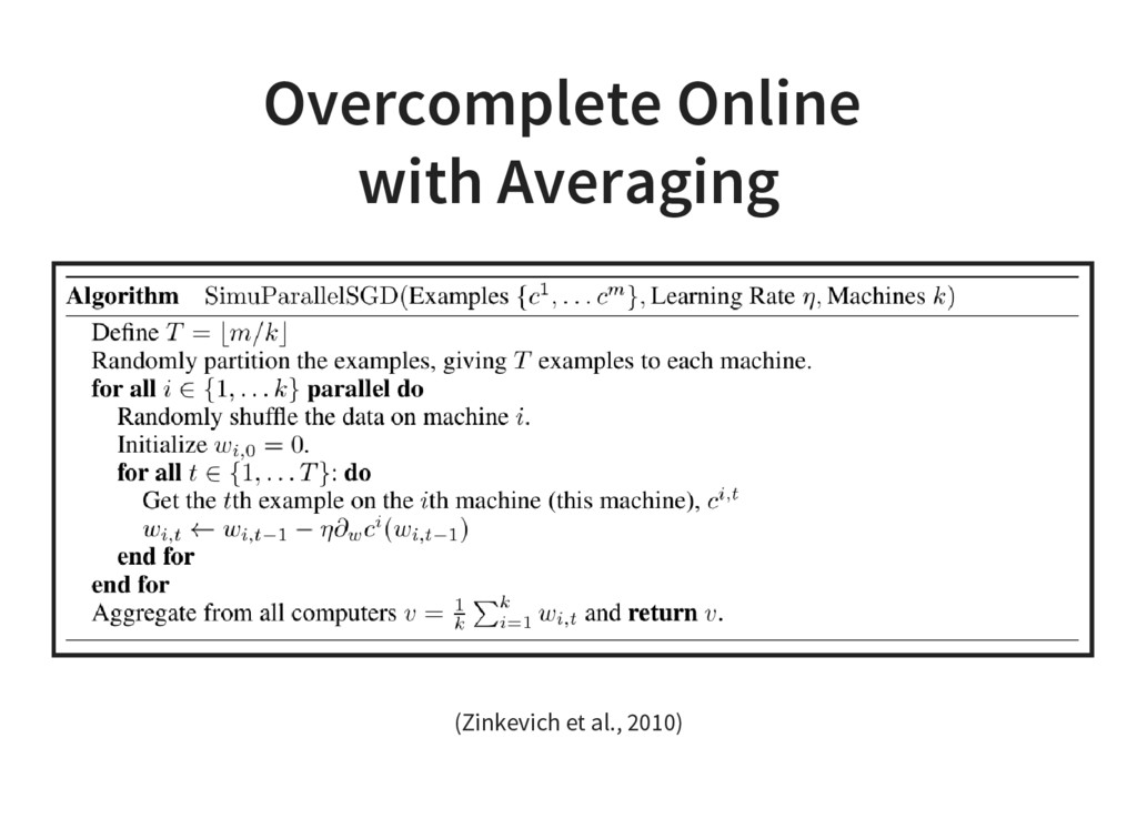
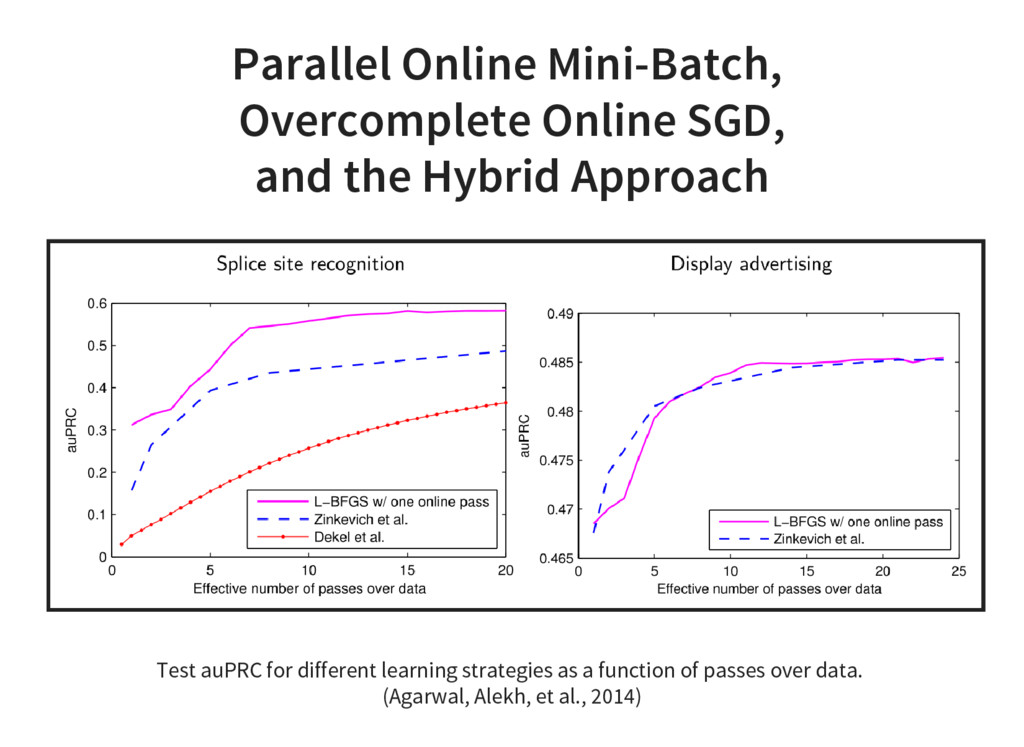
48. References [1]A. Agarwal, O. Chapelle, M. Dudík, and J. Langford, “A Reliable Effective Terascale Linear Learning System,” J. Mach. Learn. Res., vol. 15, no. 1, pp. 1111–1133, Jan. 2014. [2]M. Zinkevich, M. Weimer, L. Li, and A. J. Smola, “Parallelized stochastic gradient descent,” in Advances in neural information processing systems, 2010, pp. 2595–2603. [3]K. Weinberger, A. Dasgupta, J. Langford, A. Smola, and J. Attenberg, “Feature Hashing for Large Scale Multitask Learning,” in Proceedings of the 26th Annual International Conference on Machine Learning, New York, NY, USA, 2009, pp. 1113–1120. [4]O. Dekel, R. Gilad-Bachrach, O. Shamir, and L. Xiao, “Optimal distributed online prediction using mini-batches,” The Journal of Machine Learning Research, vol. 13, no. 1, pp. 165–202, 2012.
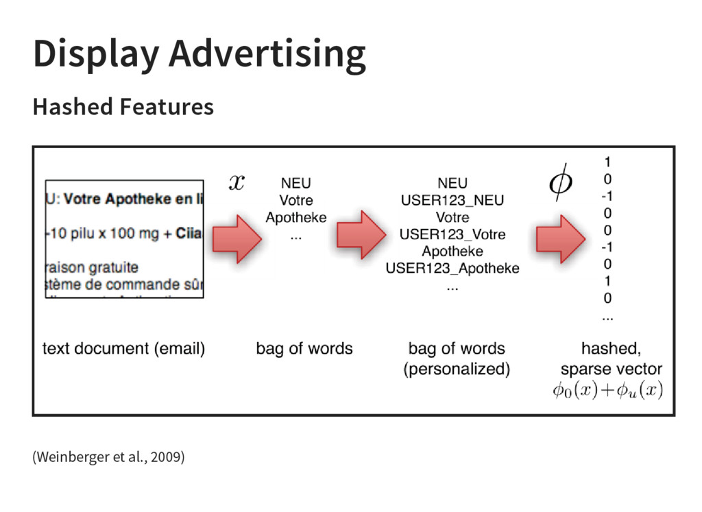
49. Hadoop-compatible AllReduce For better robustness and efficiency Use map-only Hadoop for process control and error recovery. Use AllReduce to sync state. Always save input examples in a cachefile to speed later passes. Use hashing trick to reduce input complexity.