Thinking in SQL: Going beyond “find record 5”

If you don’t understand your datastore’s strengths and weaknesses, your application is not going to scale. When is it best to carefully craft a SQL query to get exactly the information you want, and when should you just say “find(45)” and munge your data in application code?

Armed with a better understanding of SQL’s worldview you can make better decisions about what work goes in what part of your systems. We’re going to dig into a couple of example queries that do things like joining tables to themselves and intentionally creating cartesian products.

For each example you’ll see both sides of the coin:
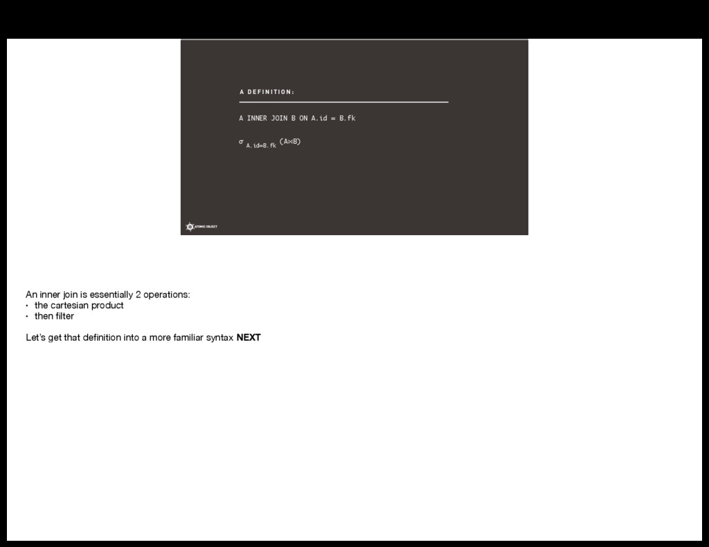
- Conceptually what each query is doing (as relational algebra)
- Practically what each query is doing (iterating over data structures in your database)

Seeing this complete picture will let you write queries that solve common real-world problems and debug the performance of your existing queries. You won’t need to be an expert in ActiveRecord, Hibernate, or another ORM, but a working knowledge of SQL will help you get the most out of this talk.

Transcript

1. Thinking in SQL M I C H A E L S W I E T O N S W I E T O N @ AT O M I C O B J E C T. C O M turn off wifi! Hello - I’m Michael Swieton. I’m a software developer at Atomic Object. We are a software design and development consultancy, and we built software for all sorts of platforms - embedded, mobile, web, server, and desktop. Today I am here to talk a bit about SQL databases because they end up being the datastore for so many of the apps that get written.
2. “… you want to build a model in your head that allows you to develop a deep understanding of the language; if you encounter a puzzle, you’ll feed it to your model and deduce the answer.” B R U C E E C K E L - T H I N K I N G I N J AVA The title of this talk is inspired by Bruce Eckel’s “Thinking in …” series of books. I hope that what I cover today will help you to improve your mental model of how SQL works. We tend to look at our problems through the lens of our tools. Often this works well - but with ORMs like ActiveRecord or Hibernate, it can be constraining.
3. How to think about joins How to think about indexes COMING ATTRACTIONS We'll cover SQL joins and some related bits - that's about 70% Then I have a largely disconnected section about indexes Everything is going to be fairly vendor-agnostic. You shouldn't have to be a SQL expert, but I won't be covering syntax at all here (despite the conference name, ha ha) I’ve made sure this talk will fit in this time slot (45 minutes) with room for questions. Feel free to ask questions I know we should have some really solid experts in the room - please feel free to heckle me and tell me all the things I'm doing wrong Finally, a disclaimer before we begin: databases are complicated, and everything I say should be mostly correct - but nothing I say will be completely 100% correct all the time.
4. J O I N
5. a INNER JOIN b a LEFT OUTER JOIN b a RIGHT OUTER JOIN b BACK TO SCHOOL A quick review: * “Give me all the pairs” * “Give me all the items on the left, and any pairings if we find a match” * “Give me all the items on the right, and any pairings if we find a match” But despite being able to regurgitate these simplified definitions, often we still think about it more like this NEXT
6. http://guides.rubyonrails.org/association_basics.html * We think about joins like "let's link record A to record B" ** Joins are just how a “has many”, “belongs to” relationship works But… these are not relational relationships. These are OO. This isn’t wrong per se - but you miss out on a lot of power if this is your only worldview of your data
7. For each A, find an associated B I N S T E A D O F: Instead of this, let’s turn it around. Instead, turn it around NEXT
8. Link every A to every B, then filter the results. T U R N I T A R O U N D : * Instead think about it as a 2 step operation: # Let's link every A to every B (that's the cartesian product) # And then let's exclude pairings that don't work * This is kind of an inversion of how we normally think - but it’s closer to the relational model Note the way we changed the language here: We stopped being imperative and talking about single records and instead are focusing on sets.
9. SELECT people.* FROM people LEFT JOIN party_invitations ON people.id = party_invitations.person_id AND party_invitations.party_id = “SyntaxCon 2016” WHERE party_invitation.id IS NULL Here’s a warm up exercise for us. I’ve got a more in-depth example, but I want to start with this. I think this query shows the problem with the idea of JOINs as “for every A, get a B”. This query finds people that have not been invited to the party. Poor them! What’s so interesting about this is that we aren’t looking for pairings: we’re looking for where we haven’t found one. Thinking about joins as just how we do “has many” makes it easy to miss a query like this, since this is the negative.
10. EXAMPLE PROBLEM What is each person’s most popular blog post? Ok, here’s problem that we’re going to dig into in depth. NEXT At Atomic, everyone writes for our blog, so this is a question we might want to ask. This form of question is very common question actually: What’s the most recent log message for each device? What’s the most expensive car in each class? Whatever. It’s easy to answer for a single person
11. SELECT * FROM blog_posts WHERE author_id=5 ORDER BY popularity DESC LIMIT 1 What is each person’s most popular blog post? It’s easy to get the answer for a single record, and we can use LINQ or Ruby’s enumerable to run the query many times - but this is inefficient.
12. What is each person’s most popular blog post? Get every post that has none more popular by author. There are other ways to get it. I’ll show you what those look like later. But right now I’m going to do it the hard way to demonstrate how I think about queries. NEXT First, I’m going to reword it a little. This is the same transformation I talked about before: • We aren’t imperatively talking about every record • Instead we have a rule that can apply declaratively to all records • And only the ones we want will fall out
13. Get every post that has none more popular by author. This looks like a join Here’s the key thing: NEXT This is a join. Rows in table blog_posts are related to other blog_posts - even though there isn’t a foreign key relationship. Ok, let’s write a query for this. NEXT
14. Get every post that has none more popular by author. SELECT * FROM blogposts p1
15. SELECT * FROM blogposts p1 LEFT OUTER JOIN blogposts p2 ON p1.views < p2.views Get every post that has none more popular by author. Joins don’t need to be a simple equality: it is any boolean expression.
16. SELECT * FROM blogposts p1 LEFT OUTER JOIN blogposts p2 ON p1.views < p2.views AND p1.employee_id=p2.employee_id Get every post that has none more popular by author.
17. SELECT * FROM blogposts p1 LEFT OUTER JOIN blogposts p2 ON p1.views < p2.views AND p1.employee_id=p2.employee_id WHERE p2.id IS NULL Get every post that has none more popular by author.
18. SELECT * FROM blogposts p1 LEFT OUTER JOIN blogposts p2 ON p1.views < p2.views AND p1.employee_id=p2.employee_id WHERE p2.id IS NULL Ok, so I hope that’s useful to see how I built that, and it’s a nice example, but it feels really opaque still.
19. Why is this so hard? A D I G R E S S I O N : Why is this so nonobvious?
20. Joins are not fundamental operations. Outer joins are very not fundamental operations. A H Y P O T H E S I S : In arithmetic, addition and subtraction are fairly fundamental. Multiplication is essentially repeated addition, but it’s still an “atom” - an effective single building block. SQL joins are not.
21. A INNER JOIN B ON A.id = B.fk σ (A⋈B) A D E F I N I T I O N : A.id=B.fk An inner join is essentially 2 operations: • the cartesian product • then filter Let’s get that definition into a more familiar syntax NEXT
22. A INNER JOIN B ON A.id = B.fk cross(A, B).filter( function(a, b) { return a.id == b.id; } ); A D E F I N I T I O N : I made up this syntax. It’s not real - I just have it here to demonstrate that there’s really two operations happening.
23. A LEFT OUTER JOIN B ON A.id = B.fk … wailing and gnashing of teeth … A D E F I N I T I O N : Now, outer joins… These are messy.
24. This is the definition on wikipedia on the “Relational Algebra” page. NEXT A left outer join involves 6 separate operations. All this work is to let you get the rows on the left (or right for a right outer join) even if there’s no match on the right (or left).
25. SELECT * FROM blogposts p1 LEFT OUTER JOIN blogposts p2 ON p1.views < p2.views AND p1.employee_id=p2.employee_id WHERE p2.id IS NULL Back to our query. There’s still a lot going on here. Here’s the question: What happens first? Let’s take another short digression. NEXT
26. SELECT * FROM blogposts p1 LEFT OUTER JOIN blogposts p2 ON p1.views < p2.views AND p1.employee_id=p2.employee_id WHERE p2.id IS NULL With *THIS* notation it is not obvious what the order of operations is. So I made one up. This isn’t official or rigorous - it’s just me writing out how I think about things and I welcome feedback.
27. SELECT * FROM blogposts p1 LEFT OUTER JOIN blogposts p2 ON p1.views < p2.views AND p1.employee_id=p2.employee_id WHERE p2.id IS NULL
28. 1. JOIN (i.e. the cartesian product) SELECT * FROM blogposts p1 LEFT OUTER JOIN blogposts p2 ON p1.views < p2.views AND p1.employee_id=p2.employee_id WHERE p2.id IS NULL Your FROM clause happens first, but within the FROM, your cartesian products happen first. Note that I’ve highlighted the JOIN but NOT the condition - it (conceptually) creates the cartesian product before it filters
29. 1. JOIN (i.e. the cartesian product) 2. Filter rows by JOIN & OUTER JOIN SELECT * FROM blogposts p1 LEFT OUTER JOIN blogposts p2 ON p1.views < p2.views AND p1.employee_id=p2.employee_id WHERE p2.id IS NULL
30. 1. JOIN (i.e. the cartesian product) 2. Filter rows by JOIN & OUTER JOIN 3. Filter rows by WHERE SELECT * FROM blogposts p1 LEFT OUTER JOIN blogposts p2 ON p1.views < p2.views AND p1.employee_id=p2.employee_id WHERE p2.id IS NULL
31. 1. JOIN (i.e. the cartesian product) 2. Filter rows by JOIN & OUTER JOIN 3. Filter rows by WHERE 4. GROUP and aggregates 5. Filter rows by HAVING 6. Filter columns by SELECT SELECT * FROM blogposts p1 LEFT OUTER JOIN blogposts p2 ON p1.views < p2.views AND p1.employee_id=p2.employee_id WHERE p2.id IS NULL Your GROUP, HAVING, and SELECT clauses all work more straightforward. The only really wacky one is the join, for reasons we discussed earlier. Ok, now let’s see how this actually works in practice for this query.
32. SELECT * FROM blogposts p1 LEFT OUTER JOIN blogposts p2 ON p1.views < p2.views AND p1.employee_id=p2.employee_id WHERE p2.id IS NULL P1.ID P1.EMP_ID P1.TITLE P1.VIEWS P2.ID P2.EMP_ID P2.TITLE P2.VIEWS 0 1 FOO 15 NULL NULL NULL NULL 1 1 BAR 30 2 2 QUX 20 So here’s that query, NEXT and here’s some data. Intentionally small dataset just for space on the slide. Let’s execute it according to my made-up SQL order of operations.
33. SELECT * FROM blogposts p1 LEFT OUTER JOIN blogposts p2 ON p1.views < p2.views AND p1.employee_id=p2.employee_id WHERE p2.id IS NULL P1.ID P1.EMP_ID P1.TITLE P1.VIEWS P2.ID P2.EMP_ID P2.TITLE P2.VIEWS 0 1 FOO 15 1 1 BAR 30 2 2 QUX 20 These are the droids we’re looking for.
34. SELECT * FROM blogposts p1 LEFT OUTER JOIN blogposts p2 ON p1.views < p2.views AND p1.employee_id=p2.employee_id WHERE p2.id IS NULL P1.ID P1.EMP_ID P1.TITLE P1.VIEWS P2.ID P2.EMP_ID P2.TITLE P2.VIEWS 0 1 FOO 15 NULL NULL NULL NULL 1 1 BAR 30 2 2 QUX 20 1 . J O I N - C A R T E S I A N P R O D U C T
35. SELECT * FROM blogposts p1 LEFT OUTER JOIN blogposts p2 ON p1.views < p2.views AND p1.employee_id=p2.employee_id WHERE p2.id IS NULL P1.ID P1.EMP_ID P1.TITLE P1.VIEWS P2.ID P2.EMP_ID P2.TITLE P2.VIEWS 0 1 FOO 15 NULL NULL NULL NULL 0 1 FOO 15 0 1 FOO 15 0 1 FOO 15 1 1 BAR 30 0 1 FOO 15 2 2 QUX 20 1 1 BAR 30 NULL NULL NULL NULL 1 1 BAR 30 0 1 FOO 15 1 1 BAR 30 1 1 BAR 30 1 1 BAR 30 2 2 QUX 20 2 2 QUX 20 NULL NULL NULL NULL 2 2 QUX 20 0 1 FOO 15 2 2 QUX 20 1 1 BAR 30 2 2 QUX 20 2 2 QUX 20 1 . J O I N - C A R T E S I A N P R O D U C T
36. SELECT * FROM blogposts p1 LEFT OUTER JOIN blogposts p2 ON p1.views < p2.views AND p1.employee_id=p2.employee_id WHERE p2.id IS NULL P1.ID P1.EMP_ID P1.TITLE P1.VIEWS P2.ID P2.EMP_ID P2.TITLE P2.VIEWS 0 1 FOO 15 NULL NULL NULL NULL 0 1 FOO 15 0 1 FOO 15 0 1 FOO 15 1 1 BAR 30 0 1 FOO 15 2 2 QUX 20 1 1 BAR 30 NULL NULL NULL NULL 1 1 BAR 30 0 1 FOO 15 1 1 BAR 30 1 1 BAR 30 1 1 BAR 30 2 2 QUX 20 2 2 QUX 20 NULL NULL NULL NULL 2 2 QUX 20 0 1 FOO 15 2 2 QUX 20 1 1 BAR 30 2 2 QUX 20 2 2 QUX 20 2 . F I LT E R B Y J O I N
37. SELECT * FROM blogposts p1 LEFT OUTER JOIN blogposts p2 ON p1.views < p2.views AND p1.employee_id=p2.employee_id WHERE p2.id IS NULL P1.ID P1.EMP_ID P1.TITLE P1.VIEWS P2.ID P2.EMP_ID P2.TITLE P2.VIEWS 0 1 FOO 15 NULL NULL NULL NULL 0 1 FOO 15 0 1 FOO 15 0 1 FOO 15 1 1 BAR 30 0 1 FOO 15 2 2 QUX 20 1 1 BAR 30 NULL NULL NULL NULL 1 1 BAR 30 0 1 FOO 15 1 1 BAR 30 1 1 BAR 30 1 1 BAR 30 2 2 QUX 20 2 2 QUX 20 NULL NULL NULL NULL 2 2 QUX 20 0 1 FOO 15 2 2 QUX 20 1 1 BAR 30 2 2 QUX 20 2 2 QUX 20 2 . F I LT E R B Y J O I N It’s actually fairly likely that your database will start its filtering here too - an index on employee is going to make this match restrict the size of the problem very effectively.
38. SELECT * FROM blogposts p1 LEFT OUTER JOIN blogposts p2 ON p1.views < p2.views AND p1.employee_id=p2.employee_id WHERE p2.id IS NULL P1.ID P1.EMP_ID P1.TITLE P1.VIEWS P2.ID P2.EMP_ID P2.TITLE P2.VIEWS 0 1 FOO 15 NULL NULL NULL NULL 0 1 FOO 15 0 1 FOO 15 0 1 FOO 15 1 1 BAR 30 0 1 FOO 15 2 2 QUX 20 1 1 BAR 30 NULL NULL NULL NULL 1 1 BAR 30 0 1 FOO 15 1 1 BAR 30 1 1 BAR 30 1 1 BAR 30 2 2 QUX 20 2 2 QUX 20 NULL NULL NULL NULL 2 2 QUX 20 0 1 FOO 15 2 2 QUX 20 1 1 BAR 30 2 2 QUX 20 2 2 QUX 20 2 . F I LT E R B Y J O I N
39. SELECT * FROM blogposts p1 LEFT OUTER JOIN blogposts p2 ON p1.views < p2.views AND p1.employee_id=p2.employee_id WHERE p2.id IS NULL P1.ID P1.EMP_ID P1.TITLE P1.VIEWS P2.ID P2.EMP_ID P2.TITLE P2.VIEWS 0 1 FOO 15 NULL NULL NULL NULL 0 1 FOO 15 0 1 FOO 15 0 1 FOO 15 1 1 BAR 30 0 1 FOO 15 2 2 QUX 20 1 1 BAR 30 NULL NULL NULL NULL 1 1 BAR 30 0 1 FOO 15 1 1 BAR 30 1 1 BAR 30 1 1 BAR 30 2 2 QUX 20 2 2 QUX 20 NULL NULL NULL NULL 2 2 QUX 20 0 1 FOO 15 2 2 QUX 20 1 1 BAR 30 2 2 QUX 20 2 2 QUX 20 2 . 5 . F I N I S H T H E J O I N As we discussed earlier, outer joins are complicated. An OUTER JOIN will give you NULLs where there are no matches, but since we had matches here, we don’t need this tuple.
40. SELECT * FROM blogposts p1 LEFT OUTER JOIN blogposts p2 ON p1.views < p2.views AND p1.employee_id=p2.employee_id WHERE p2.id IS NULL P1.ID P1.EMP_ID P1.TITLE P1.VIEWS P2.ID P2.EMP_ID P2.TITLE P2.VIEWS 0 1 FOO 15 NULL NULL NULL NULL 0 1 FOO 15 0 1 FOO 15 0 1 FOO 15 1 1 BAR 30 0 1 FOO 15 2 2 QUX 20 1 1 BAR 30 NULL NULL NULL NULL 1 1 BAR 30 0 1 FOO 15 1 1 BAR 30 1 1 BAR 30 1 1 BAR 30 2 2 QUX 20 2 2 QUX 20 NULL NULL NULL NULL 2 2 QUX 20 0 1 FOO 15 2 2 QUX 20 1 1 BAR 30 2 2 QUX 20 2 2 QUX 20 3 . F I LT E R B Y W H E R E
41. SELECT * FROM blogposts p1 LEFT OUTER JOIN blogposts p2 ON p1.views < p2.views AND p1.employee_id=p2.employee_id WHERE p2.id IS NULL P1.ID P1.EMP_ID P1.TITLE P1.VIEWS P2.ID P2.EMP_ID P2.TITLE P2.VIEWS 0 1 FOO 15 NULL NULL NULL NULL 0 1 FOO 15 0 1 FOO 15 0 1 FOO 15 1 1 BAR 30 0 1 FOO 15 2 2 QUX 20 1 1 BAR 30 NULL NULL NULL NULL 1 1 BAR 30 0 1 FOO 15 1 1 BAR 30 1 1 BAR 30 1 1 BAR 30 2 2 QUX 20 2 2 QUX 20 NULL NULL NULL NULL 2 2 QUX 20 0 1 FOO 15 2 2 QUX 20 1 1 BAR 30 2 2 QUX 20 2 2 QUX 20 G R O U P, H AV I N G , A G G R E G AT E S The remaining steps are for queries with GROUP BY, HAVING, or aggregate functions, so we don’t change anything for those.
42. SELECT * FROM blogposts p1 LEFT OUTER JOIN blogposts p2 ON p1.views < p2.views AND p1.employee_id=p2.employee_id WHERE p2.id IS NULL P1.ID P1.EMP_ID P1.TITLE P1.VIEWS P2.ID P2.EMP_ID P2.TITLE P2.VIEWS 0 1 FOO 15 NULL NULL NULL NULL 0 1 FOO 15 0 1 FOO 15 0 1 FOO 15 1 1 BAR 30 0 1 FOO 15 2 2 QUX 20 1 1 BAR 30 NULL NULL NULL NULL 1 1 BAR 30 0 1 FOO 15 1 1 BAR 30 1 1 BAR 30 1 1 BAR 30 2 2 QUX 20 2 2 QUX 20 NULL NULL NULL NULL 2 2 QUX 20 0 1 FOO 15 2 2 QUX 20 1 1 BAR 30 2 2 QUX 20 2 2 QUX 20 And now we’re finished with the top records per employee. Let’s pause for a second there. What do you think of that? Do you believe me that this works?
43. SELECT * FROM ( SELECT *, RANK(views) OVER (PARTITION BY employee_id) AS post_rank FROM blogposts ) WHERE post_rank = 1; Now, I just showed you the hard way to do it. Here’s the easy way, and honestly a lot more powerful. You probably should be using this solution when you have this problem. I’m not going to dig into this much - go read your database server’s manual. And here’s another NEXT
44. SELECT DISTINCT ON (employee_id) * FROM blogposts ORDER BY employee_id, views DESC; And here’s an even simpler way of doing it. If you understand the hard way of doing it, you’re going to have the mental model you’ll need to understand a lot of other and more complicated queries, so that’s why I wanted to cover it. But this is a good lesson too: You should check out your tools and see what they’ll allow. They often support much more elegant solutions than we may have been stuck with twenty years ago.
45. SELECT people.* FROM people LEFT JOIN party_invitations ON people.id = party_invitations.person_id AND party_invitations.party_id = “SyntaxCon 2016” WHERE party_invitation.id IS NULL 1. Make the cartesian product 2. Filter to desired pairings and NULLs 3. Then select rows from the result Ok let’s go back to the beginning for a moment. NEXT This is the same query we looked at first. Now, having walked through that execution, it should be clear how this one works. Let’s mark it up a bit. NEXT NEXT NEXT That’s all I wanted to say about joins before we move on.
46. I N D E X E S We use indexes to make things faster. But if you’re going to be even remotely effective you need to know a little bit more about how they work. Let’s dig in.
47. A redundant copy Of some columns Of all rows In sorted order That is automatically maintained as data is updated AN INDEX IS: Here’s my definition of an index: Ok, now let’s see how it works.
48. L. NAME F. NAME GENDER DOB NALL KEVIN MALE 1983-03-25 EMERSON ALYSIA FEMALE 1979-03-23 PINO ADRIANE FEMALE 2002-07-24 GAGNON GRACIA FEMALE 2015-09-15 EVERS CHARLES MALE 1995-04-15 NOBLES MAIA FEMALE 1992-06-23 AIKEN LORINDA FEMALE 1964-05-05 MARINO MARVIN MALE 1980-08-12 SELECT * FROM people WHERE last_name=‘EVERS’ L. NAME AIKEN EMERSON EVERS GAGNON MARINO NALL NOBLES PINO Here’s some data. Suppose we want to query it. NEXT Now this isn’t that hard of a question for us to answer, but it’s still harder than it needs to be, and without some ordering to the records it quickly becomes impossible to answer manually as our dataset gets bigger. Let’s add an index on last name. NEXT Things to note: • The index is in order: this allows us to search according to its keys • And it references the original source data. An indirection must happen when we want rows not in the index! • In practice this will be a B-tree or equivalent search-oriented structure - displayed here as a list for ease • It’s a redundant copy of the data - this must be kept up to date as things change! So if we want to answer this query, we can very efficiently search the index.
49. L. NAME F. NAME GENDER DOB NALL KEVIN MALE 1983-03-25 EMERSON ALYSIA FEMALE 1979-03-23 PINO ADRIANE FEMALE 2002-07-24 GAGNON GRACIA FEMALE 2015-09-15 EVERS CHARLES MALE 1995-04-15 NOBLES MAIA FEMALE 1992-06-23 AIKEN LORINDA FEMALE 1964-05-05 MARINO MARVIN MALE 1980-08-12 SELECT * FROM people WHERE last_name=‘EVERS’ L. NAME AIKEN EMERSON EVERS GAGNON MARINO NALL NOBLES PINO So if we want to answer this query, we can very efficiently search the index. It’ll find the record in the index, and then follow a pointer back to the source table for the remaining columns.
50. L. NAME F. NAME GENDER DOB NALL KEVIN MALE 1983-03-25 EMERSON ALYSIA FEMALE 1979-03-23 PINO ADRIANE FEMALE 2002-07-24 GAGNON GRACIA FEMALE 2015-09-15 EVERS CHARLES MALE 1995-04-15 NOBLES MAIA FEMALE 1992-06-23 AIKEN LORINDA FEMALE 1964-05-05 MARINO MARVIN MALE 1980-08-12 SELECT * FROM people WHERE last_name LIKE ‘E%’ AND gender=‘Female’ L. NAME AIKEN EMERSON EVERS GAGNON MARINO NALL NOBLES PINO Ok, let’s try this again with a new query. NEXT Now the index will quickly get us a smaller set of records to match: NEXT
51. L. NAME F. NAME GENDER DOB NALL KEVIN MALE 1983-03-25 EMERSON ALYSIA FEMALE 1979-03-23 PINO ADRIANE FEMALE 2002-07-24 GAGNON GRACIA FEMALE 2015-09-15 EVERS CHARLES MALE 1995-04-15 NOBLES MAIA FEMALE 1992-06-23 AIKEN LORINDA FEMALE 1964-05-05 MARINO MARVIN MALE 1980-08-12 L. NAME AIKEN EMERSON EVERS GAGNON MARINO NALL NOBLES PINO SELECT * FROM people WHERE last_name LIKE ‘E%’ AND gender=‘Female’ But the index does not get us all the way: we need to go back to the source data before we can filter it to the one matching row.
52. L. NAME F. NAME GENDER DOB NALL KEVIN MALE 1983-03-25 EMERSON ALYSIA FEMALE 1979-03-23 PINO ADRIANE FEMALE 2002-07-24 GAGNON GRACIA FEMALE 2015-09-15 EVERS CHARLES MALE 1995-04-15 NOBLES MAIA FEMALE 1992-06-23 AIKEN LORINDA FEMALE 1964-05-05 MARINO MARVIN MALE 1980-08-12 L. NAME AIKEN EMERSON EVERS GAGNON MARINO NALL NOBLES PINO SELECT * FROM people WHERE last_name LIKE ‘E%’ AND gender=‘Female’ But the index does not get us all the way: we need to go back to the source data before we can filter it to the one matching row.
53. L. NAME F. NAME GENDER DOB NALL KEVIN MALE 1983-03-25 EMERSON ALYSIA FEMALE 1979-03-23 PINO ADRIANE FEMALE 2002-07-24 GAGNON GRACIA FEMALE 2015-09-15 EVERS CHARLES MALE 1995-04-15 NOBLES MAIA FEMALE 1992-06-23 AIKEN LORINDA FEMALE 1964-05-05 MARINO MARVIN MALE 1980-08-12 SELECT * FROM people WHERE first_name=‘Kevin’ L. NAME AIKEN EMERSON EVERS GAGNON MARINO NALL NOBLES PINO At this point you should be getting a clue to the main indexing principle: the database can only take advantage of the indexed columns in the order you give it. The index is sorted by last name, so it obviously does not help us answer this question NEXT However, less obviously, even this index doesn’t help any NEXT
54. L. NAME F. NAME GENDER DOB NALL KEVIN MALE 1983-03-25 EMERSON ALYSIA FEMALE 1979-03-23 PINO ADRIANE FEMALE 2002-07-24 GAGNON GRACIA FEMALE 2015-09-15 EVERS CHARLES MALE 1995-04-15 NOBLES MAIA FEMALE 1992-06-23 AIKEN LORINDA FEMALE 1964-05-05 MARINO MARVIN MALE 1980-08-12 SELECT * FROM people WHERE first_name=‘Kevin’ L. NAME F. NAME AIKEN LORINDA EMERSON ALYSIA EVERS CHARLES GAGNON GRACIA MARINO MARVIN NALL KEVIN NOBLES MAIA PINO ADRIANE The index is sorted by the columns you put in it in that order. Merely having the column in an index does not help you, if you are not also matching on the first column of the index! More examples in a moment. For example, NEXT
55. CoreyCurtin KevinNall AlysiaEmerson AdrianePino GraciaGagnon CharlesEvers MaiaNobles LorindaAiken AN INDEX ON: first_name, last_name WHERE first_name=‘Gracia’ AND last_name=‘Gagnon’ HELPS A LOT WITH: Suppose we had an index on first_name, last_name. Here’s a binary tree representation of the data in the index. Note that I’ve run the keys together - this is how I think about indexes. Since you can’t query by the second or third column or nth column of a compound index, I think this is a good way to think about it. Now your database doesn’t use a naive binary tree for indexes. But I do think it’s a good way to visualize it. Please forgive my crappy binary tree here, but I hope it gets the idea across. Looking at this, it should be obvious that it will help with a value like this. NEXT
56. CoreyCurtin KevinNall AlysiaEmerson AdrianePino GraciaGagnon CharlesEvers MaiaNobles LorindaAiken AN INDEX ON: first_name, last_name GraciaGagnon HELPS A LOT WITH: It’s essentially just walking the tree looking for matches on this value.
57. CoreyCurtin KevinNall AlysiaEmerson AdrianePino GraciaGagnon CharlesEvers MaiaNobles LorindaAiken AN INDEX ON: first_name, last_name GraciaGagnon HELPS A LOT WITH: It’s essentially just walking the tree looking for matches on this value.
58. CoreyCurtin KevinNall AlysiaEmerson AdrianePino GraciaGagnon CharlesEvers MaiaNobles LorindaAiken AN INDEX ON: first_name, last_name WHERE last_name=‘Gagnon’ DOES NOTHING FOR: Now at the same time, it’s clear that this is just not something
59. AN INDEX ON: first_name, last_name HELPS A LOT WITH: WHERE first_name = ‘Bob’ WHERE first_name = ‘Bob’ AND last_name = ‘Jones’ WHERE first_name = ‘Bob’ AND last_name LIKE ‘J%’ WHERE first_name = ‘B%’ WHERE first_name = ‘B%’ AND last_name LIKE ‘J%’ DOES NOTHING FOR: WHERE last_name LIKE ‘J%’ WHERE first_name LIKE ‘%ob’ Let me summarize: Here is a different example index. In this case, we do first and last name.
60. Any column Other stuff… sometimes WHAT CAN BE INDEXED? Most of the time, the index contains the values in a column. However, you can sometimes index expressions: Function results for example. In particular, Postgres does include mechanisms for indexing json columns effectively. That’s not going to be a magical way to speed up access to anything, but if there’s a specific key in the json column that is a condition in queries, you can index a specific path or expression in the document.
61. WHY ISN’T IT USING MY INDEX? Your database will estimate costs and pick the cheapest strategy. Now, let’s assume that it’s possible for it to be using the index. E.g. you have a possible prefix match. NEXT The database has a cost estimator that uses a number of techniques to guess what the best strategy is. It’s not using your index because it disagrees with you. Here’s an example
62. SELECT * FROM people WHERE last_name=‘EVERS’ Not using an index: 1. Scan the table 2. Filter on last_name=‘EVERS’ (TABLE ROW READ COST) * (NUMBER OF ROWS) Let’s look at this query again. We could do it just by reading rows in the table NEXT And it guesses the cost like this. NEXT And if we fill in what we know (and what the database knows), it looks like this NEXT
63. SELECT * FROM people WHERE last_name=‘EVERS’ Not using an index: 1. Scan the table 2. Filter on last_name=‘EVERS’ (TABLE ROW READ COST) * 8
64. SELECT * FROM people WHERE last_name=‘EVERS’ Using an index on last_name: 1. Index range scan on last_name=‘EVERS’ 2. Read remaining columns from source table (INDEX READ COST) * (ESTIMATED NUMBER OF ROWS) + (TABLE ROW READ COST) * (ESTIMATED NUMBER OF ROWS) Now, is this cheaper than a full scan or not? NEXT Well… maybe NEXT
65. SELECT * FROM people WHERE last_name=‘EVERS’ Using an index on last_name: 1. Index range scan on last_name=‘EVERS’ 2. Read remaining columns from source table (INDEX READ COST) * 1+ (TABLE ROW READ COST) * 1 Your database keeps statistics about the data. This is summary data - designed to be small so it can look at it quickly to make decisions, and it’s cached and not 100% up to date all the time. Based on these statistics, it can estimate that an equality comparison on last_name will result in a single match and it’s going to do this instead of the full scan. Here’s how it knows that
66. Postgres has some good “system tables” that you can look at. I copied this query (and the one from earlier) from their documentation. We’re querying on DOB and gender, so let’s look at those: • First, look at the n_distinct column: • The “-1” means that every value is unique • If it were a positive integer, it’s the number of unique values • And the -0.22 is a proportion: It means that for gender, there’s one unique value for every 5 records. Our test data had 3 males and 5 females, so that seems close. • It also knows some of the most common values for each column. Given this, your database can make a guess at the rows we will get back.
67. SELECT * FROM people WHERE dob < ‘1990-01-01’ Not using an index: 1. Scan the table 2. Filter on dob < ‘1990-01-01’ (TABLE ROW READ COST) * (NUMBER OF ROWS) Here’s a different condition. Now this one is interesting. Again, we could do it just by reading rows in the table and it will have comparable costs.
68. SELECT * FROM people WHERE dob < ‘1990-01-01’ Not using an index: 1. Scan the table 2. Filter on dob < ‘1990-01-01’ (TABLE ROW READ COST) * 8 Here’s a different condition. Now this one is interesting. Again, we could do it just by reading rows in the table and it will have comparable costs.
69. SELECT * FROM people WHERE dob < ‘1990-01-01’ Using an index on dob 1. Index range scan on dob < ‘1990-01-01’ 2. Read remaining columns from source table (INDEX READ COST) * (ESTIMATED NUMBER OF ROWS) + (TABLE ROW READ COST) * (ESTIMATED NUMBER OF ROWS) And here’s the index version. Everything here looks the same, but let’s fill in values.
70. SELECT * FROM people WHERE dob < ‘1990-01-01’ Using an index on dob 1. Index range scan on dob < ‘1990-01-01’ 2. Read remaining columns from source table (INDEX READ COST) * 8 + (TABLE ROW READ COST) * 8 And here’s the index version. Everything here looks the same, but let’s fill in values. In this case, it doesn’t know how many rows will match so it assumes all of them will. In this case it’s going to probably prefer a full table scan or try using a different index.
71. SELECT * FROM people WHERE last_name = ‘Evers’ AND gender=‘Male’ Cost for using either index: (INDEX READ COST) * (ESTIMATED NUMBER OF ROWS) + (TABLE ROW READ COST) * (ESTIMATED NUMBER OF ROWS) One last example. Suppose in this case we have two indexes: one on last_name, and one on gender. In this case, the formula for cost is the same. But let’s look more closely NEXT
72. SELECT * FROM people WHERE last_name = ‘Evers’ AND gender=‘Male’ Cost for using last_name: (INDEX READ COST) * 1 + (TABLE ROW READ COST) * 1 So no surprise, if we use last_name we estimate 1 row and it’s fairly cheap.
73. SELECT * FROM people WHERE last_name = ‘Evers’ AND gender=‘Male’ Cost for using gender: (INDEX READ COST) * (8 * 0.22) + (TABLE ROW READ COST) * (8 * 0.22) But here’s what it looks like if we use gender Note that extra factor in there: For gender, we know we don’t have a lot of unique values. So it scales it according to it’s statistics about how much that value narrows the field.
74. Prefix match Prefer indexes with higher cardinality INDEXING PRINCIPLES Reviewing, we earlier covered the first principle of indexes: you can use an index if its first key is in your query. And now we can add a second principle: indexes on more varied columns are better. An index on a value like gender usually only reduce your result set by 50%. But a value like date of birth might get you down to a single row.
75. http://use-the-index-luke.com http://modern-sql.com/ FURTHER READING These are two web sites by Markus Winand. They have some really fantastic content for understanding indexes and new SQL features. There’s a lot out there and your database probably has some tools you’re not using that would let you better understand your queries and perhaps write better ones, so you should understand that. I hope that what I’ve covered today is gives you some helpful heuristics to start with. Thanks!
76. M I C H A E L S W I E T O N S W I E T O N @ AT O M I C O B J E C T. C O M Hello - I’m Michael Swieton. I’m a software developer at Atomic Object. We are a software design and development consultancy, and we built software for all sorts of platforms - embedded, mobile, web, server, and desktop. Today I am here to talk a bit about SQL databases because they end up being the datastore for so many of the apps that get written.