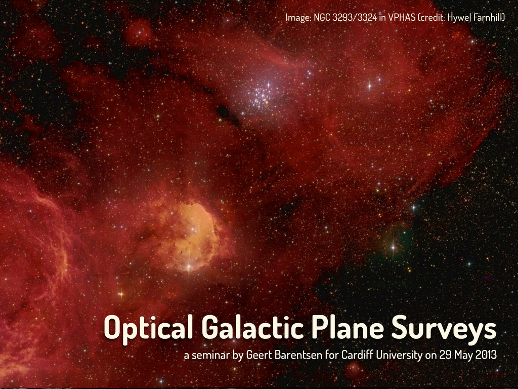
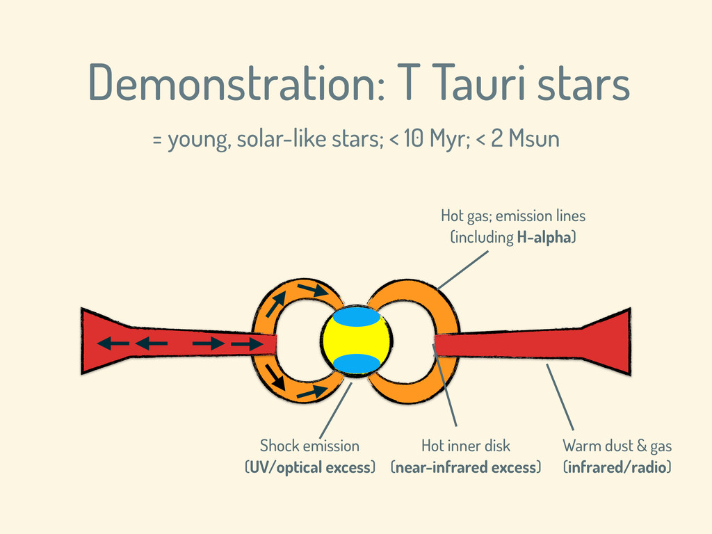
entire Galactic Plane in visible light. 2. Scientific rationale These projects are a necessary counterpart to infrared surveys. Also a key complement to Gaia. 3. Demonstration Discovery and parameter inference of young stars using survey photometry.
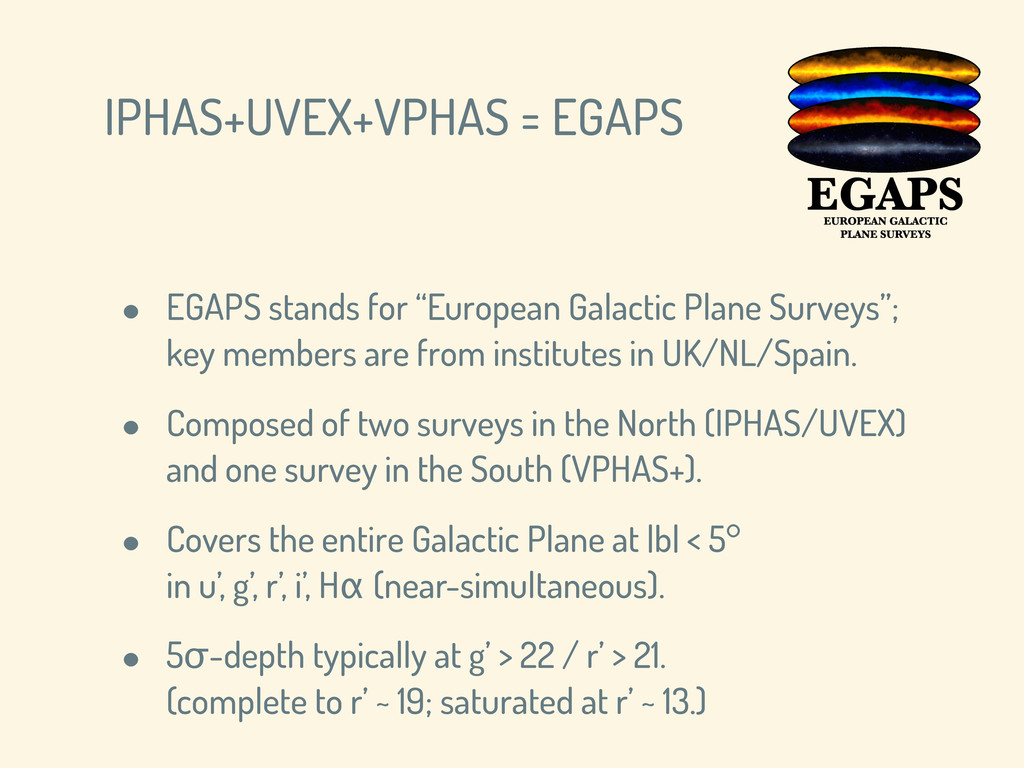
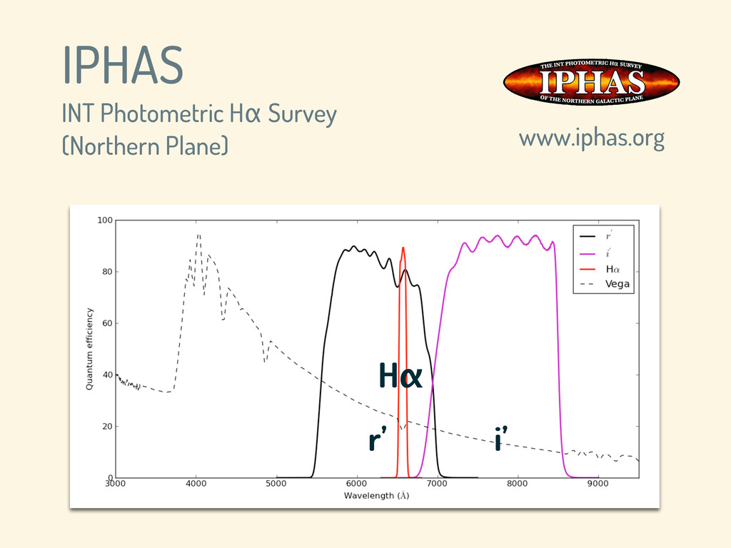
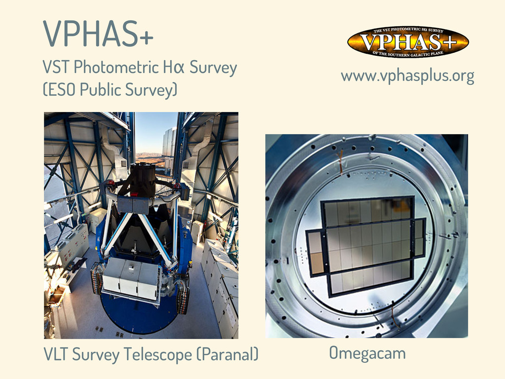
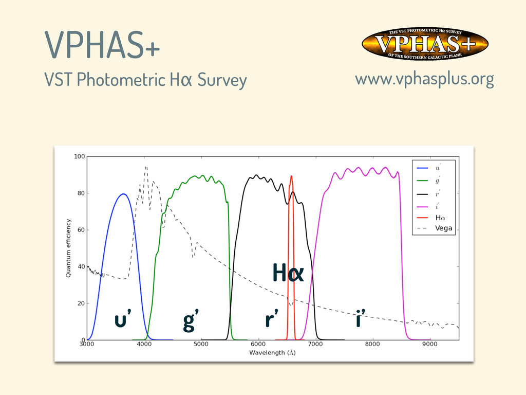
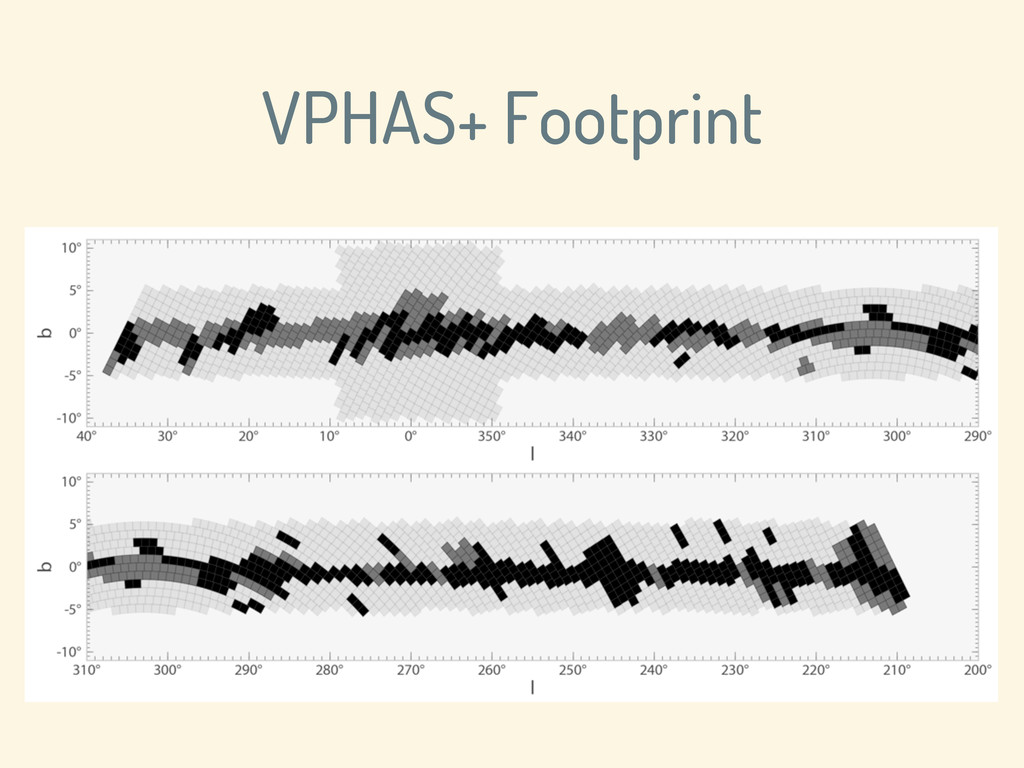
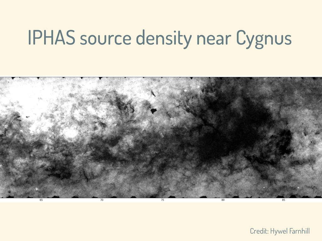
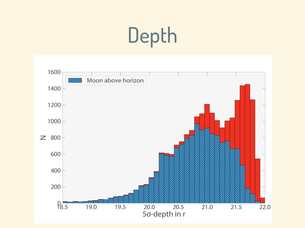
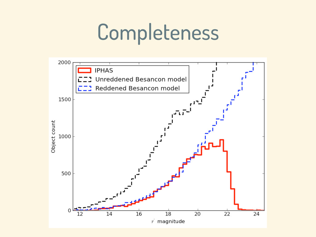
Surveys”; key members are from institutes in UK/NL/Spain. • Composed of two surveys in the North (IPHAS/UVEX) and one survey in the South (VPHAS+). • Covers the entire Galactic Plane at |b| < 5° in u’, g’, r’, i’, Hα (near-simultaneous). • 5σ-depth typically at g’ > 22 / r’ > 21. (complete to r’ ~ 19; saturated at r’ ~ 13.)
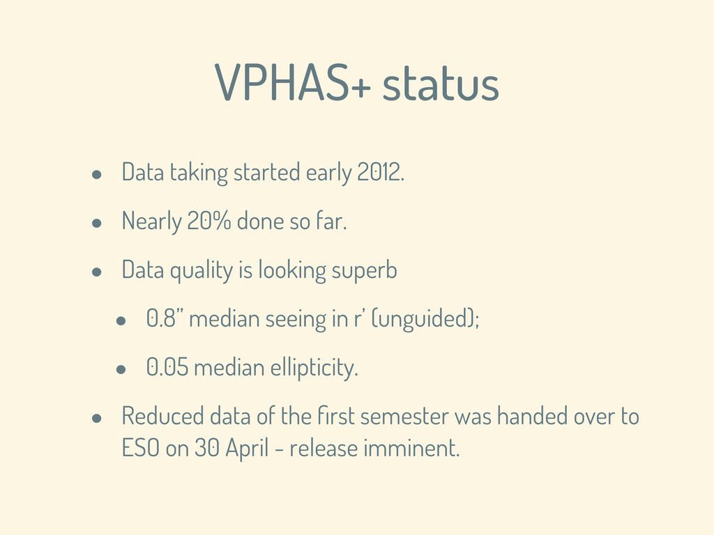
20% done so far. • Data quality is looking superb • 0.8” median seeing in r’ (unguided); • 0.05 median ellipticity. • Reduced data of the first semester was handed over to ESO on 30 April - release imminent.
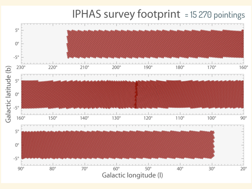
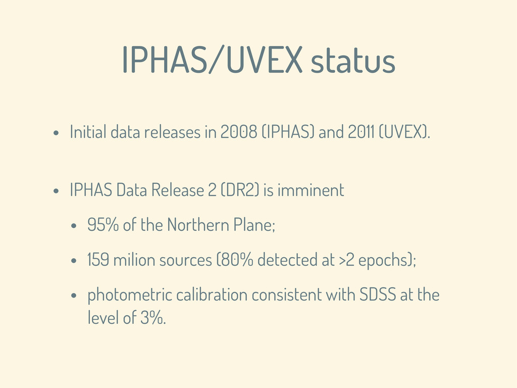
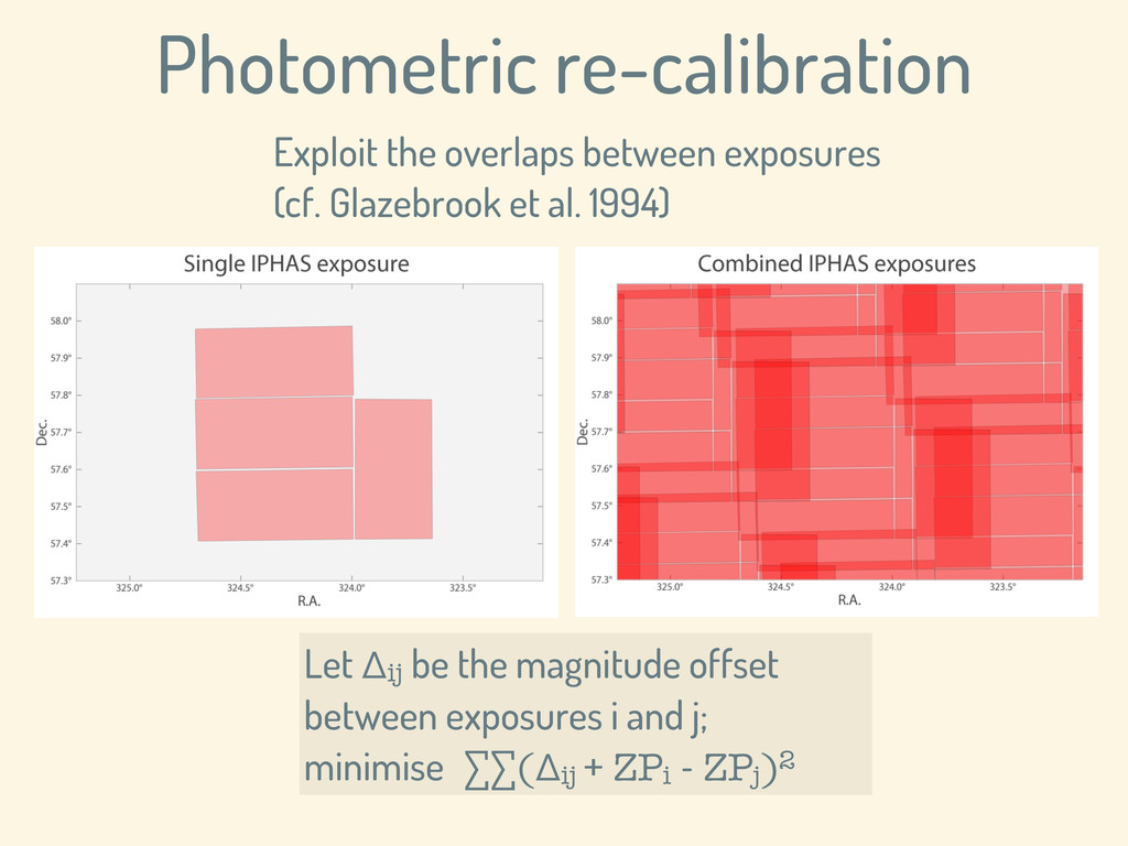
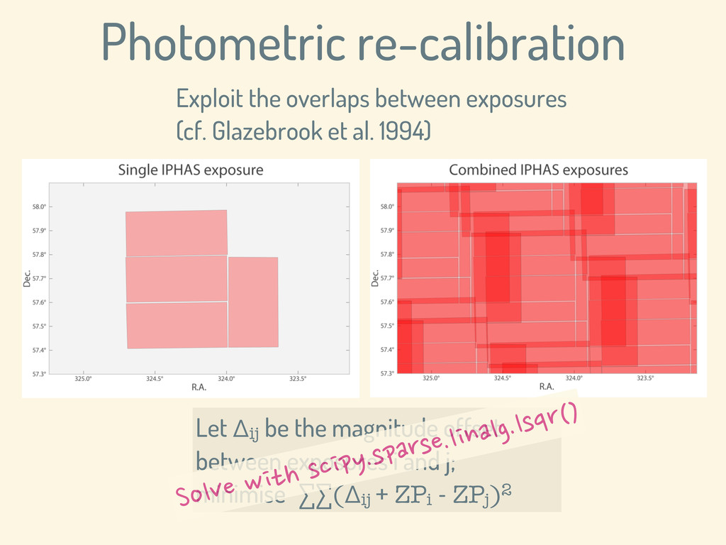
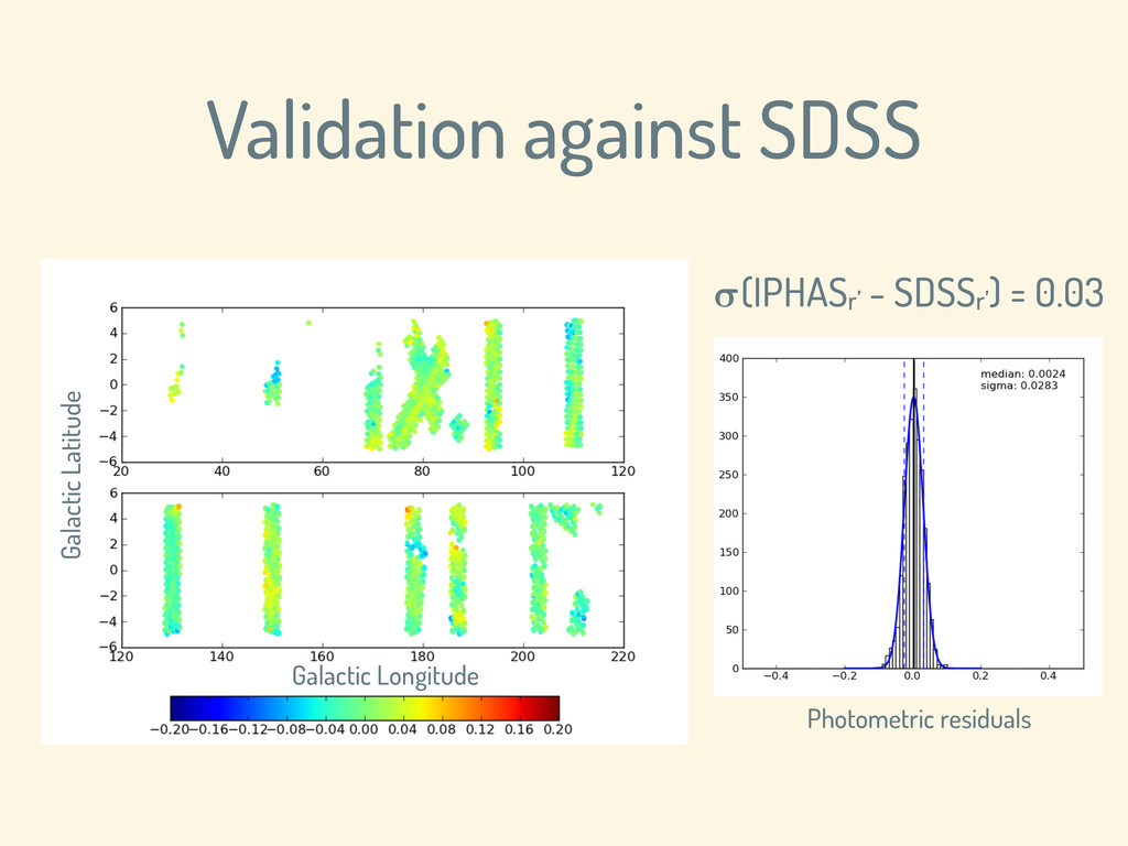
2011 (UVEX). • IPHAS Data Release 2 (DR2) is imminent • 95% of the Northern Plane; • 159 milion sources (80% detected at >2 epochs); • photometric calibration consistent with SDSS at the level of 3%.
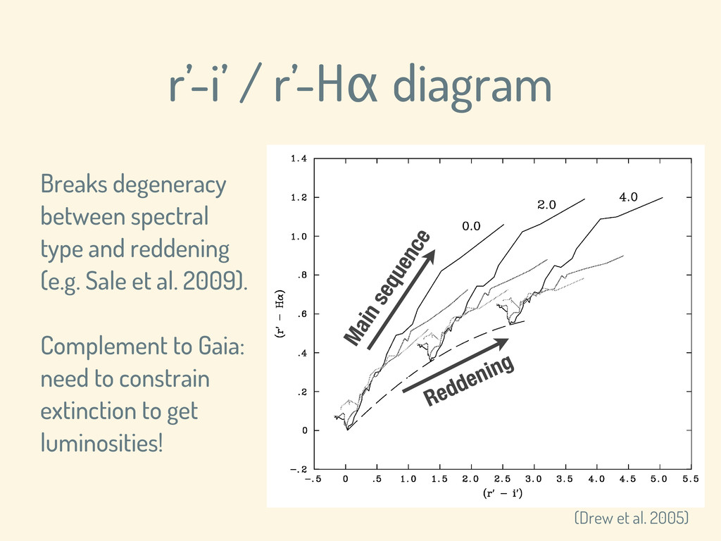
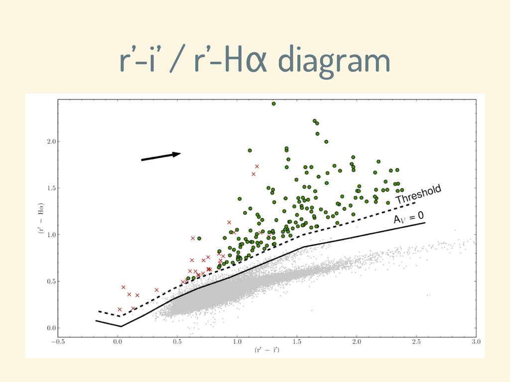
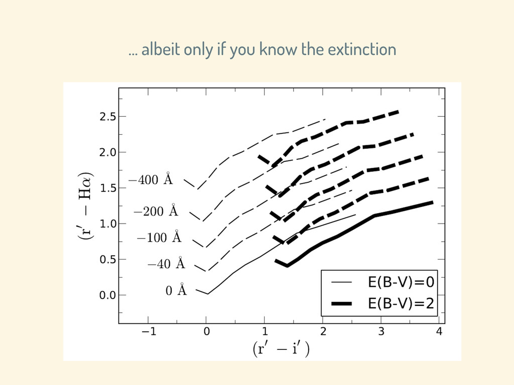
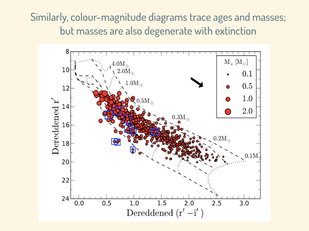
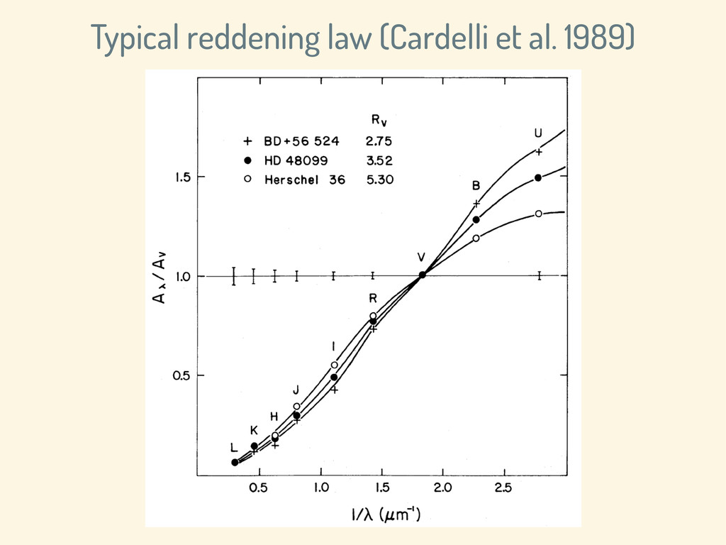
sequence Reddening Breaks degeneracy between spectral type and reddening (e.g. Sale et al. 2009). Complement to Gaia: need to constrain extinction to get luminosities!
entire Galactic Plane in visible light. 2. Scientific rationale These projects are a necessary counterpart to infrared surveys. Also a key complement to Gaia. 3. Demonstration Discovery and parameter inference of young stars using survey photometry.
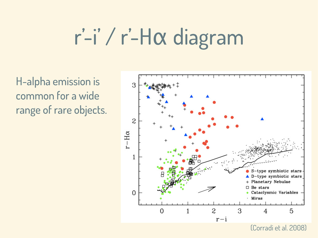
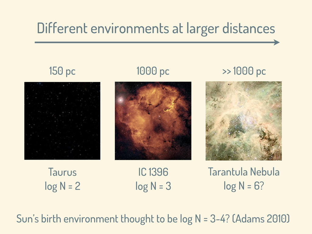
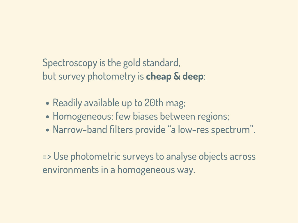
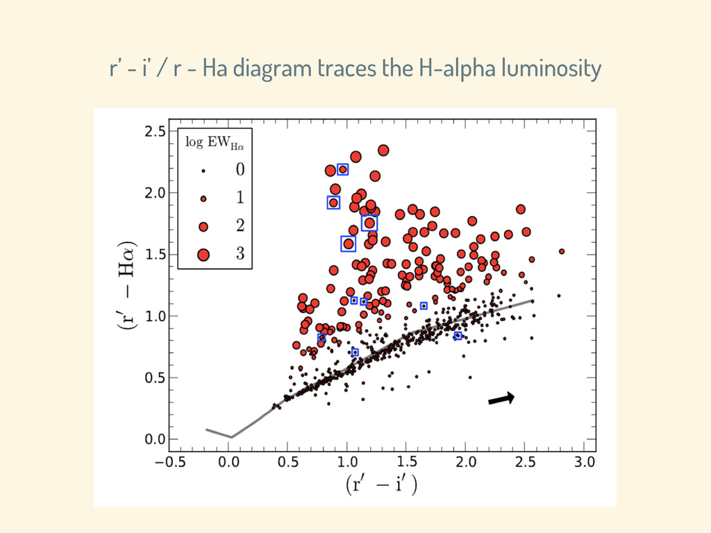
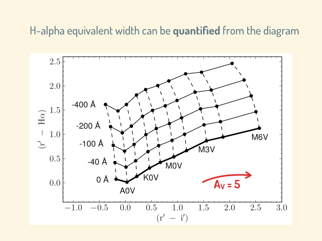
& deep: • Readily available up to 20th mag; • Homogeneous: few biases between regions; • Narrow-band filters provide “a low-res spectrum”. => Use photometric surveys to analyse objects across environments in a homogeneous way.
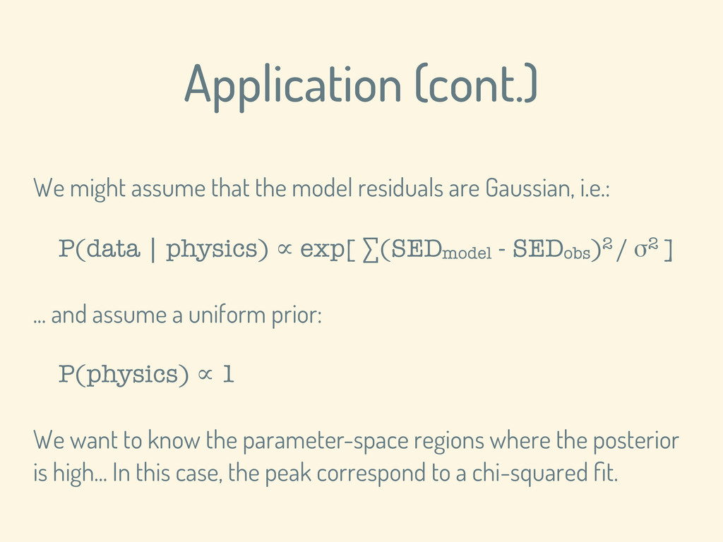
Gaussian, i.e.: P(data | physics) ∝ exp[ ∑(SEDmodel - SEDobs)2 / σ2 ] ... and assume a uniform prior: P(physics) ∝ 1 We want to know the parameter-space regions where the posterior is high... In this case, the peak correspond to a chi-squared fit.
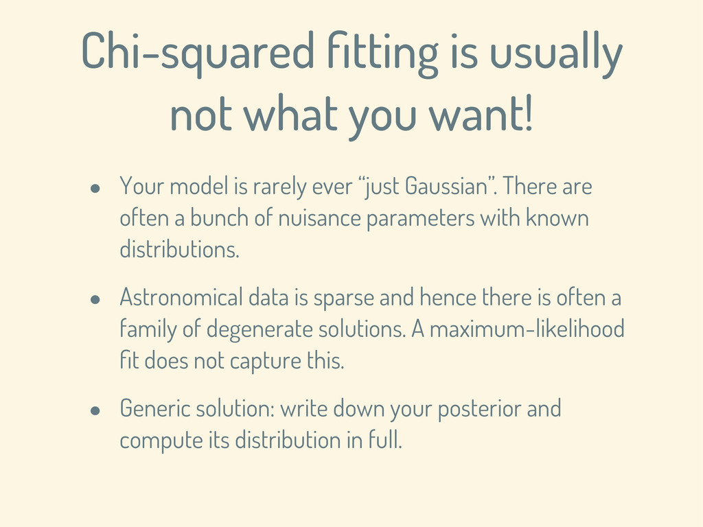
model is rarely ever “just Gaussian”. There are often a bunch of nuisance parameters with known distributions. • Astronomical data is sparse and hence there is often a family of degenerate solutions. A maximum-likelihood fit does not capture this. • Generic solution: write down your posterior and compute its distribution in full.
u’, g’, r’, i’, H-alpha. • Get in touch if you would like to use the data, or keep an eye out for “IPHAS DR2”. • Take-away message: Python and Graphical Probabilistic Models are key tools for mining surveys.
Nijmegen (UVEX PI) University of Cambridge (pipeline) University of Graz Other members: Instituto de Astrofísica de Canarias, Harvard/Smithsonian CfA, University College London, Imperial College London, University of Warwick, University of Manchester, University of Southampton, Armagh Observatory, Macquarie University, Tautenburg Observatory, ESTEC, University of Valencia. Key individuals: Janet Drew, Hywel Farnhill, Geert Barentsen, Robert Greimel, Mike Irwin, Eduardo Gonzalez-Solares, Romano Corradi, Paul Groot (UVEX lead), Danny Steeghs.