Building graphs to discover information by David Martínez at Big Data Spain 2015

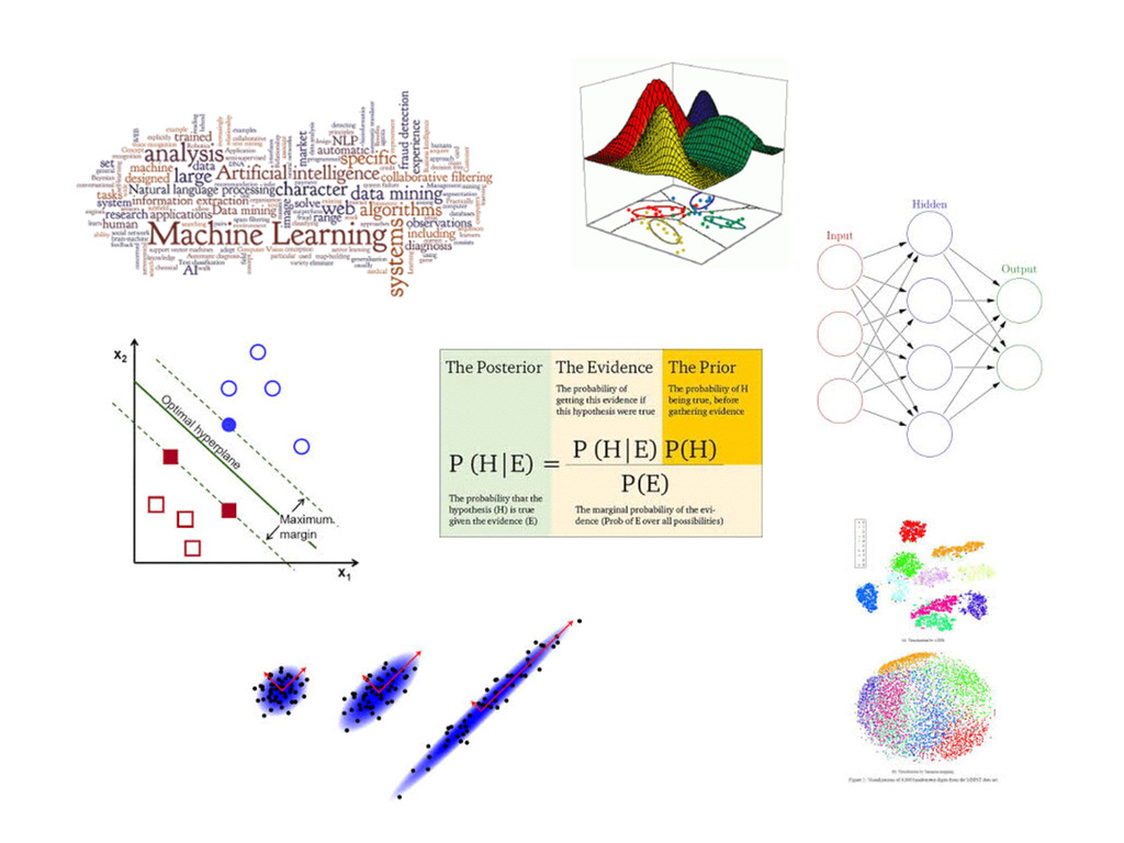
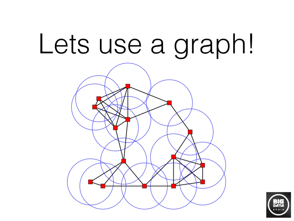
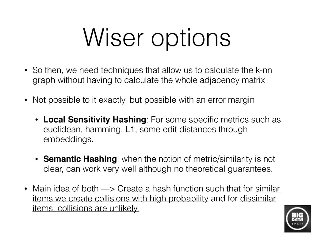
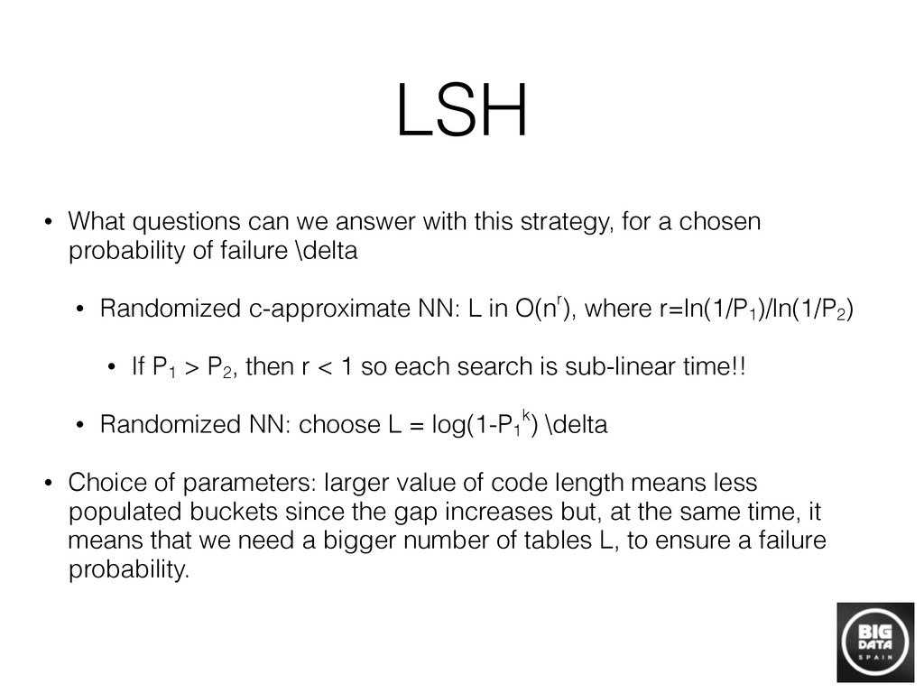
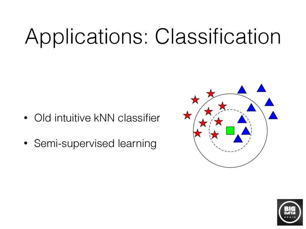
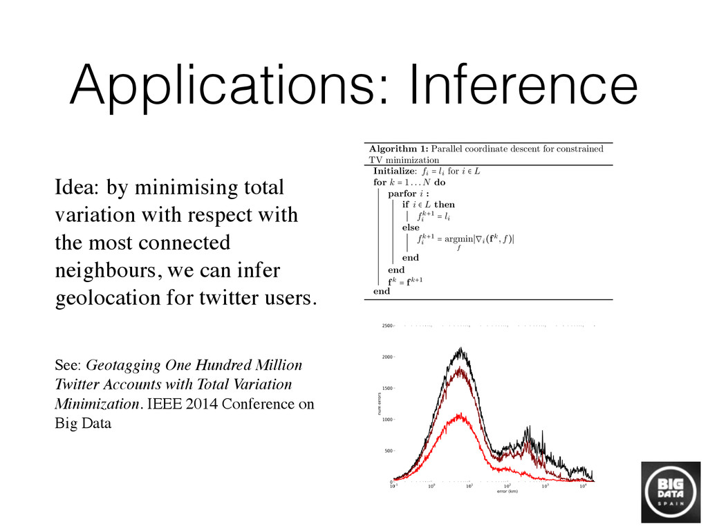
The basic challenge of a data scientist is to unveil information from raw data. Traditional machine learning algorithms have treated “pure” data analytics situations that should comply with a set of restrictions, such as access to labels, a clear prediction objective… However, the reality in practice shows that, due to the wide spread of data science nowadays, the exception is the norm and it is usual to encounter situations that depend on gathering information from raw data which lacks any kind of structure, or objective that classic approaches assume. In these situations, building a graph that encodes the information we are trying to unveil is the most intuitive place to start or even the only one feasible when we lack any field knowledge or previously stated aim. Unfortunately, building a graph when the number of nodes is huge from scratch is a challenging task computationally, and requires some approximations to make it feasible. In this review, we will talk about the most standard way of building those graphs in practice, and how to exploit them to solve data science tasks.

Session presented at Big Data Spain 2015 Conference
15th Oct 2015
Kinépolis Madrid
http://www.bigdataspain.org
Event promoted by: http://www.paradigmatecnologico.com
Abstract: http://www.bigdataspain.org/program/thu/slot-11.html#spch11.2

Transcript

2. Building graphs to discover information Dr. David Martinez Rego Big Data Spain 2015
3. Data science? • Every once in a while you hear the same question in the office, discussion,… • But.. what is a data scientist? • Of course the response is usually vague, but my definition (from the ML point of view) • Do whatever you can to transform raw data in information that carries some business value?
4. Acme project: Day 1 • After the first handshake, reality! • The team is usually handed data which has not been prepared for any learnable task • The aim (BV) is not clear or present at all • Many books talking about design strategies • Context, need, vision, outcome (Max Shron)
7. Labels? Prior knowledge? Exploration? Scale?
8. ?
9. Lets use a graph!
10. Lets use a graph!
11. What can I do? • Find structure in the information • Connected components • Hubs • Infer information (more on this later…) • Clustering • Classification • Anomaly detection • Many more…
12. Anywhere? • Scalable graph algorithms are behind many of the recent biggest developments • PageRank, social networks, medical research, DevOps, … • So, is there an extra mile? • All these cases have something in common, they take the graph for granted, • it is already given by the problem • it is highly sparse • it carries business value
13. Anywhere? • What about the case where the graph is not explicit • That case carries more work, since it we have to figure out • how to encode individuals in a way that the graph carries the information we want • how to build the graph itself is a challenging problem!!
14. Anywhere? • Naïve algorithm! • for i=1..N • for j=1..N • M[i,j] = sim(d[i], d[j]) • prune(graph) If we have around 1 million entities, the calculation is way bigger than the whole set of tweets in a year.
15. Wiser options • So then, we need techniques that allow us to calculate the k-nn graph without having to calculate the whole adjacency matrix • Not possible to it exactly, but possible with an error margin • Local Sensitivity Hashing: For some specific metrics such as euclidean, hamming, L1, some edit distances through embeddings. • Semantic Hashing: when the notion of metric/similarity is not clear, can work very well although no theoretical guarantees. • Main idea of both —> Create a hash function such that for similar items we create collisions with high probability and for dissimilar items, collisions are unlikely.
16. LSH 8 Kristen Grauman and Rob Fergus D t b hr r n Database hr 1 …r b << n X i Series of b randomized LSH functions Colliding instances are searched 110101 << n Q functions Q 111101 110111 hr 1 …r b Hash table: Similar instances collide, w.h.p. Query Fig. 5 Locality Sensitive Hashing (LSH) uses hash keys constructed so as to guarantee collision is more likely for more similar examples [33, 23]. Once all database items have been hashed into the table(s), the same randomized functions are applied to novel queries. One exhaustively searches only those examples with which the query collides. counters some of these shortcomings, and allows a user to explicitly control the similarity search accuracy and search time tradeoff [23]. Kristen Grauman & Rob Fergus Local Sensitivity Hashing
17. LSH • LSH relies on the existence of LSH Family of functions for a given metric. • A family H is (R, cR, P1, P2)-sensitive if for any two points p and q! • if |p-q| < R, then P[h(p) == h(q)] > P1 • if |p-q| > cR, then P[h(p) == h(q)] < P2 where h is independently randomly selected from family H and P1 > P2
18. LSH • The effect emerges from basic probability phenomenon • For a hash function length m, there is a p1 m probability of two close points to collide • On the other hand, the probability of far apart points to collide is p2 m • If p1 > p2 then the gap would increase with moderate code sizes • Unfortunately, when designing the LSH we can not always achieve a high p1 • Build several tables with the same strategy so the probability of finding an approximate nearest neighbour increases by a union bound.
19. LSH input set into a bucket g j (p), for j = 1,…,L. Since the total number of buckets may be large, we retain only the nonempty buckets by resort- ing to (standard) hashing3 of the values g j (p). In this way, the data structure uses only O(nL) memory cells; note that it suffices that the buckets store the pointers to data points, not the points themselves. To process a query q, we scan through the buckets g 1 (q),…, g L (q), and retrieve the points stored in them. After retrieving the points, we com- 3See [16] for more details on hashing. log 1 – P1 k ␦ so that (1 – P 1 k)L ≤ ␦, then any R-neighbor of q is returned by the algorithm with probability at least 1 – ␦. How should the parameter k be chosen? Intuitively, larger values of k lead to a larger gap between the probabilities of collision for close points and far points; the probabilities are P 1 k and P 2 k, respectively (see Figure 3 for an illustration). The benefit of this amplification is that the hash functions are more selective. At the same time, if k is large then P 1 k is small, which means that L must be sufficiently large to ensure that an R-near neighbor collides with the query point at least once. Preprocessing: 1. Choose L functions g j , j = 1,…L, by setting g j = (h 1, j , h 2, j ,…h k, j ), where h 1, j ,…h k, j are chosen at random from the LSH family H. 2. Construct L hash tables, where, for each j = 1,…L, the jth hash table contains the dataset points hashed using the function g j . Query algorithm for a query point q: 1. For each j = 1, 2,…L i) Retrieve the points from the bucket g j (q) in the jth hash table. ii) For each of the retrieved point, compute the distance from q to it, and report the point if it is a correct answer (cR-near neighbor for Strategy 1, and R-near neighbor for Strategy 2). iii) (optional) Stop as soon as the number of reported points is more than LЈ. Fig. 2. Preprocessing and query algorithms of the basic LSH algorithm. COMMUNICATIONS OF THE ACM January 2008/Vol. 51, No. 1 119
20. LSH • What questions can we answer with this strategy, for a chosen probability of failure \delta • Randomized c-approximate NN: L in O(nr), where r=ln(1/P1 )/ln(1/P2 ) • If P1 > P2 , then r < 1 so each search is sub-linear time!! • Randomized NN: choose L = log(1-P1 k) \delta • Choice of parameters: larger value of code length means less populated buckets since the gap increases but, at the same time, it means that we need a bigger number of tables L, to ensure a failure probability.
21. Next steps… • So, we can find an R-NN in sub-linear time, and now what? • Unfortunately, from this point on the theory is less revealing, but practical results are good. • What if I cannot encode my problem with one of those metrics?
22. Semantic Hashing • It makes use of the most internal representation of an autoencoder as a hash function • Training process • First we train a set of stacked RBMs in a layer wise manner RBM RBM RBM
23. Semantic Hashing • Training process • First we train a set of stacked RBMs in a layer wise manner • Then we fine tune an unrolled version of the original network N bit code
24. Semantic Hashing • Search process • Build a hash table by locating each element in its corresponding bucket • Get the elements inside the n-hamming ball N bit code
25. Applications: Clustering • Correlation clustering! • Allows us to find groups without specifying a priori the number of them (or the shape) + + + + + + + + + + + + + + + + + + - - - -
26. Applications: Clustering • Correlation clustering! • Implementations • Pivot algorithm: 3-approximation • Parallel version: requires log (n)2 iterations + + + + + + + + + + + + + + + + + + - - - - Pick random pivot i ∈ V! Set , V'=Ø! For all j ∈ V, j ≠ i;! If (i,j) ∈ E+ then! Add j to C! Else (If (i,j) ∈ E−)! Add j to V'! Let G' be the subgraph induced by V'! Return clustering C,CC-Pivot(G')! • While the instance is non-empty 1.Let A be its current maximum positive degree 2.2. Activate each element independently with probability e/A 3.Deactivate all the active elements that are connected through a positive edge to other active elements 4.The remaining active nodes become pivots 5.Create one cluster for each pivot (breaking ties randomly)
27. Applications: Anomaly detection • Local outlier factor (LOF)! • An anomaly is a point that has an abnormal low density when compared with other points similar to it
28. Applications: Classification • Old intuitive kNN classifier • Semi-supervised learning
29. Applications: Inference Idea: by minimising total variation with respect with the most connected neighbours, we can infer geolocation for twitter users. See: Geotagging One Hundred Million Twitter Accounts with Total Variation Minimization. IEEE 2014 Conference on Big Data Figure 6: Histogram of tweets as a function of activity level. For each group of users described in fig. 4 and fig. 5 we collected the total number of tweets generated by the group. Despite the high number of inactive users, the bulk of tweets are generated by active Twitter users, indicating the impor- tance of geotagging active accounts. Figure 7: Histogram of errors with di↵erent restrictions on the maximum allowable geographic dispersion of each user’s (a) CDF of the geographic distance between friends (b) CDF of the geographic distance between a user and their geographically closest friend Figure 2: Study of contact patterns between users who reveal their location via GPS. Subgraphs of GPS users are taken from the, the bidirectional @mention network (blue), bidirectional @mention network after filtering edges for triadic closures (green), and the complete unidirectional @mention network (black). In (a), we see that the distances spanned by reciprocated @mentions (blue and green) are smaller than those spanned by any @mention (black). In (b), we see that users often have at least one online social tie with a geographically nearby user. The subgraph sizes are: 19 , 515 , 278 edges and 3 , 972 , 321 nodes (green), 20 , 576 , 189 edges and 4 , 488 , 759 node (blue), 100 , 126 , 247 edges and 5 , 648 , 220 nodes (black). We suspect these results would be even stronger if more GPS data were available. well-aligned with geographic distance, we restrict our atten- tion to GPS-known users and study contact patterns between them in fig. 2. Users with GPS-known locations make up only a tiny por- tion of our @mention networks. Despite the relatively small amount of data, we can still see in fig. 2 that online social ties typically form between users who live near each other and that a majority of GPS-known users have at least one GPS-known friend within 10km. The optimization (1) models proximity of connected users. Unfortunately, the total variation functional is nondi↵eren- tiable and finding a global minimum is thus a formidable chal- lenge. We will employ “parallel coordinate descent” [25] to solve (1). Most variants of coordinate descent cycle through the domain sequentially, updating each variable and commu- nicating back the result before the next variable can update. The scale of our data necessitates a parallel approach, pro- hibiting us from making all the communication steps required by a traditional coordinate descent method. At each iteration, our algorithm simultaneously updates each user’s location with the l 1-multivariate median of their friend’s locations. Only after all updates are complete do we communicate our results over the network. At iteration k , denote the user estimates by fk and the variation on the i th node by ￿∇ i ( fk ,f )￿ = ￿ j wijd ( f,fk j ) (6) Parallel coordinate descent can now be stated concisely in alg. 1. The argument that minimizes (6) is the l 1-multivariate me- dian of the locations of the neighbours of node i . By placing this computation inside the parfor of alg. 1, we have repro- duced the Spatial Label Propagation algorithm of [12] as a Algorithm 1: Parallel coordinate descent for constrained TV minimization Initialize : fi = li for i ∈ L for k = 1 ...N do parfor i : if i ∈ L then fk +1 i = li else fk +1 i = argmin f ￿∇ i ( fk ,f )￿ end end fk = fk +1 end coordinate descent method designed to minimize total varia- tion. 3.4 Individual Error Estimation The vast majority of Twitter users @mention with geograph- ically close users. However, there do exist several users who have amassed friends dispersed around the globe. For these users, our approach should not be used to infer location. We use a robust estimate of the dispersion of each user’s friend locations to infer accuracy of our geocoding algorithm. Our estimate for the error on user i is the median absolute deviation of the inferred locations of user i ’s friends, com- puted via (3). With a dispersion restriction as an additional parameter, , our optimization becomes min f ￿∇ f ￿ subject to fi = li for i ∈ L and max i ∼ ∇ fi < (7)
30. Applications (many more) Blossom algorithm Shortest paths Search Algorithms Bipartite Minimum Cut
31. Wrap up! Raw data Extract Features Locality Hashing Navigate An. detection Clustering Inference
32. Building graphs to discover information Dr. David Martinez Rego Big Data Spain 2015