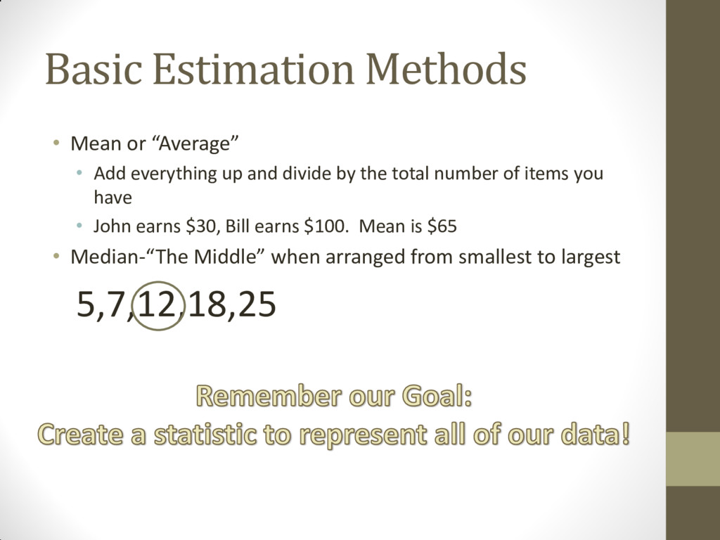
up and divide by the total number of items you have • John earns $30, Bill earns $100. Mean is $65 • Median-“The Middle” when arranged from smallest to largest 5,7,12,18,25
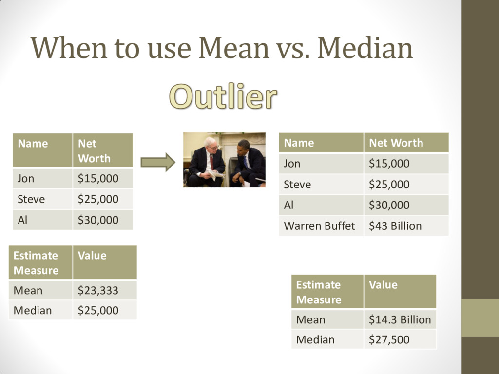
$15,000 Steve $25,000 Al $30,000 Estimate Measure Value Mean $23,333 Median $25,000 Name Net Worth Jon $15,000 Steve $25,000 Al $30,000 Warren Buffet $43 Billion Estimate Measure Value Mean $14.3 Billion Median $27,500
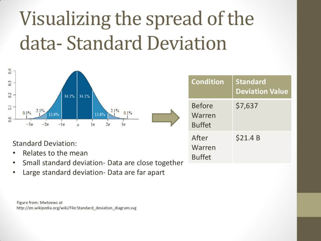
Mwtoews at http://en.wikipedia.org/wiki/File:Standard_deviation_diagram.svg Standard Deviation: • Relates to the mean • Small standard deviation- Data are close together • Large standard deviation- Data are far apart Condition Standard Deviation Value Before Warren Buffet $7,637 After Warren Buffet $21.4 B
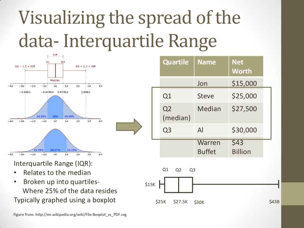
http://en.wikipedia.org/wiki/File:Boxplot_vs_PDF.svg Interquartile Range (IQR): • Relates to the median • Broken up into quartiles- Where 25% of the data resides Typically graphed using a boxplot Quartile Name Net Worth Jon $15,000 Q1 Steve $25,000 Q2 (median) Median $27,500 Q3 Al $30,000 Warren Buffet $43 Billion $15K $27.5K $25K $30K $43B Q1 Q2 Q3
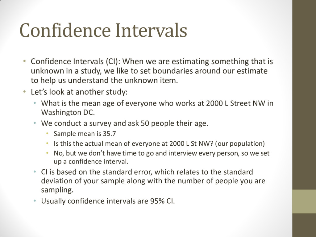
something that is unknown in a study, we like to set boundaries around our estimate to help us understand the unknown item. • Let’s look at another study: • What is the mean age of everyone who works at 2000 L Street NW in Washington DC. • We conduct a survey and ask 50 people their age. • Sample mean is 35.7 • Is this the actual mean of everyone at 2000 L St NW? (our population) • No, but we don’t have time to go and interview every person, so we set up a confidence interval. • CI is based on the standard error, which relates to the standard deviation of your sample along with the number of people you are sampling. • Usually confidence intervals are 95% CI.
our mean age at 2000 L St NW is between 32.7 and 38.7. What does this mean? • Our “best guess” for our study is that the true population mean lies within the 95% Confidence Interval of 32.7-38.7 • If we repeated our survey 100 times, 95 times out a 100 we would have an estimate where our CI contains the true population mean.
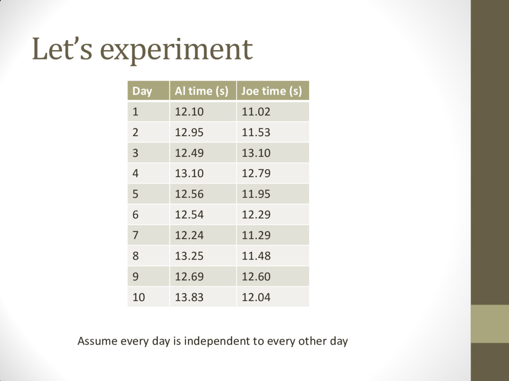
about data • Statisticians draw conclusions by testing a hypothesis • What is a scientific hypothesis? • It is a guess about what you think will happen with your data based upon past observations. Almost always it is something that is not interesting in the data. It is often called the Null Hypothesis. • For example: • Null Hypothesis: Al and Frank type at the same rate • Null Hypothesis: Drug A and Drug B reduce breast cancer tumors by the same amount • Null Hypothesis: Al and Joe both run the 100 m dash in the same amount of time • Then we test whether the null hypothesis is true
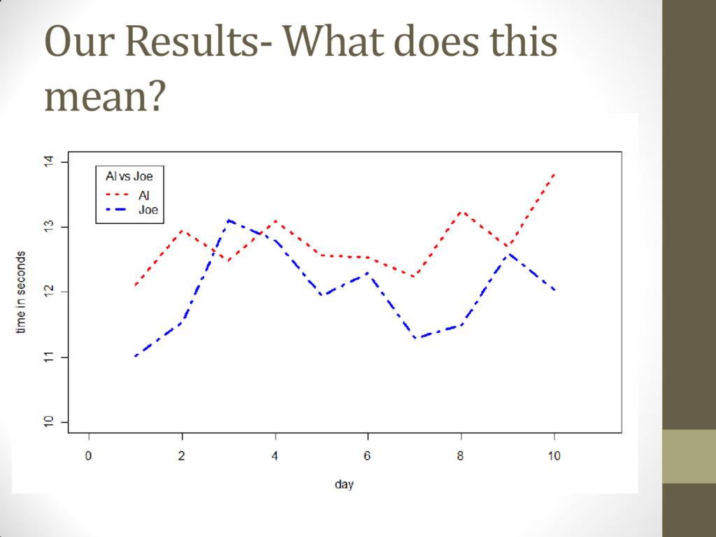
to know, is Al’s mean running time for the 100m dash different than Joe’s mean running time for the same race? • In statistical notation: • Null Hypothesis (H0 ): Al and Joe run the 100 m dash in the same amount of time (they have the same mean running time). • Alternative Hypothesis (HA ): Al and Joe do not run the 100 m dash in the same amount of time (their mean running times are not equal).
in a way that is standardized so others can follow and reproduce our results • One of the easiest tests is a t test • In a t test, you compare whether the mean of one group (Al’s running times) is equal to the mean of another group (Joe’s running times) • Remember, our Null Hypothesis (H0 ): Al and Joe run the 100 m dash in the same amount of time (they have the same mean running time). • Our significance level is α of 0.05
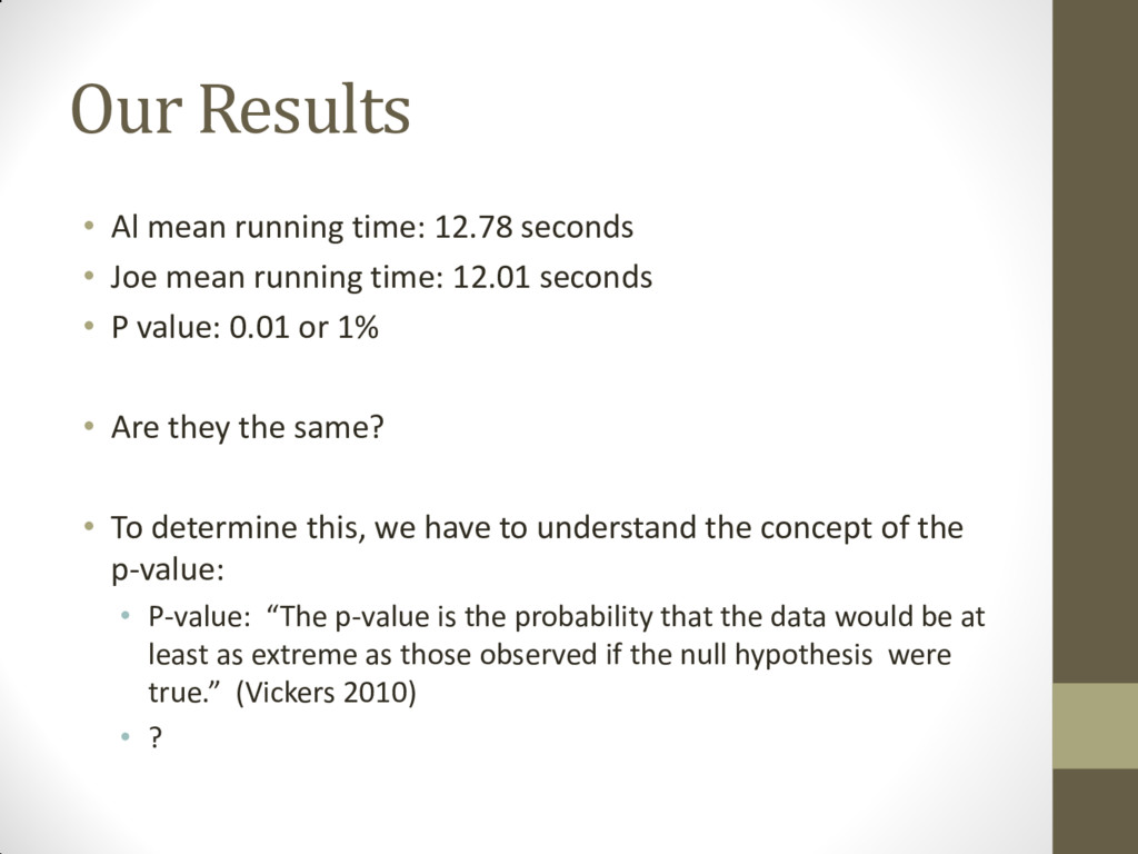
Joe mean running time: 12.01 seconds • P value: 0.01 or 1% • Are they the same? • To determine this, we have to understand the concept of the p-value: • P-value: “The p-value is the probability that the data would be at least as extreme as those observed if the null hypothesis were true.” (Vickers 2010) • ?
There is a 1% probability that we would see data at least as extreme as the data we collected from Al and Joe and they would still have the same mean 100 m dash running time. • In other words: Al and Joe may have the same mean running time, but according to our statistical methods, we would only see data like these 1/100 times if that were the case. • So what do we say? • Since 1/100 is not very likely, we reject our null hypothesis that the mean running times of Al and Joe are equal and accept our alternative hypothesis that they are not equal. • Conclusion: Al and Joe do not have equal mean running times of the 100 m dash • But…… • Could we be wrong?
our sample, this could have been the 1% of the time where the data are very extreme…we are not 100% certain. • But, based upon our statistical significance level of 0.05, we feel confident enough to reject our null hypothesis • And anyone reading our research will know our p-value=0.01 so they can draw the same conclusion as we can.
hypothesis when we should not have rejected it. • Example: Let’s say Al and Joe do have the same mean running times for the 100 m dash, but we said that they do not and we made a mistake. We made a Type I error (Probability of making a Type I error is call α). • Type II Error: Fail to reject the null hypothesis when we should have rejected it. • Example: Let’s say that Al and Joe do not have the same mean running times for the 100 m dash, but we said that they do have the same mean running times. We made a Type II error (Probability of making a Type II error is called β).
when the null hypothesis is false. • Power is 1-β (also known as sensitivity) • Power depends on variation and sample size • A “Power Analysis” is what typically helps determine how many subjects should be sampled in a study. • “The findings were not significant because we believe the study was underpowered.” • Translation: The researchers didn’t have enough samples in the study, probably because of budget constraints, and that is why they did not get a p-value low enough to reject the null hypothesis.
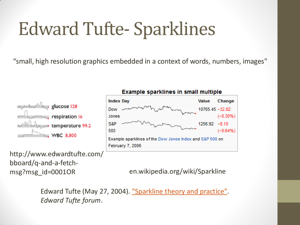
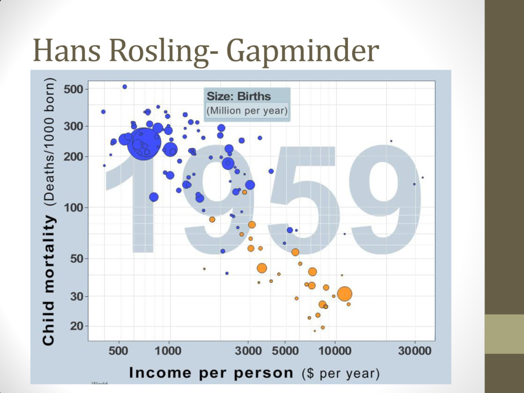
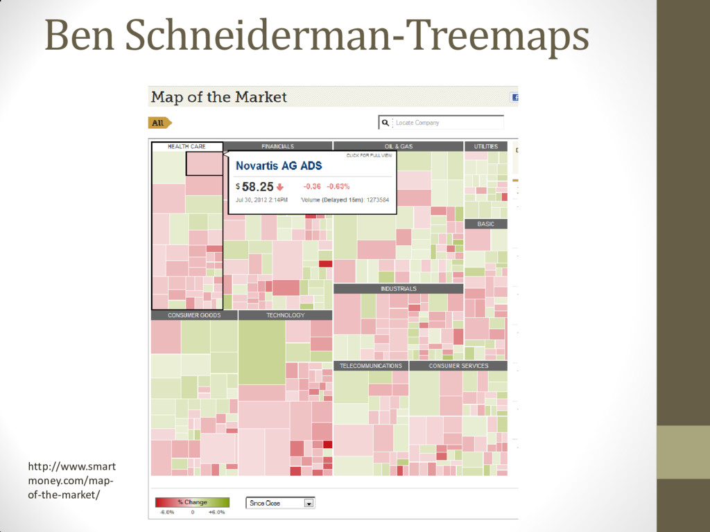
the “democratization” of analysis, being able to manipulate and visualize data is a major competitive advantage. • Definite trend in taking the analysis that statisticians perform and working with designers to visualize it. • Some of my favorite data visualizers: • Edward Tufte (http://www.edwardtufte.com/) • Nathan Yau (http://flowingdata.com) • Nancy Duarte (http://www.duarte.com/) • Hans Rosling (http://www.gapminder.org/) • Ben Schneiderman (http://www.cs.umd.edu/~ben/)
context of words, numbers, images" Edward Tufte (May 27, 2004). "Sparkline theory and practice". Edward Tufte forum. en.wikipedia.org/wiki/Sparkline http://www.edwardtufte.com/ bboard/q-and-a-fetch- msg?msg_id=0001OR
risk • Probability of exposure vs. Probability of non-exposure • 20 times as many smokers have cancer compared to non-smokers • Odds Ratio (O.R.) • Odds of outcome with experimental group vs. odds of outcome with control group • Typically used in clinical trials and with logistic regression • OR of 2 means the experimental group has twice the odds of the outcome compared to the control group.
trial for a man who pickpocketed a wallet: • Null Hypothesis: The man is innocent • Probability of committing a Type I error (α): “Beyond a reasonable doubt.” You set your alpha level based upon what will get you to beyond a reasonable doubt. If you set it wrong, you could send an innocent man to prison. • Probability of committing a Type II error (β): Can be adjusted as you receive more evidence in the case. For example if you have 1 witness claim to see the man pickpocket, that may not be enough to reject the null hypothesis. If you have 100 witnesses claim to see a man pickpocket, you have reduced the probability of a Type II error. • Why do we care?
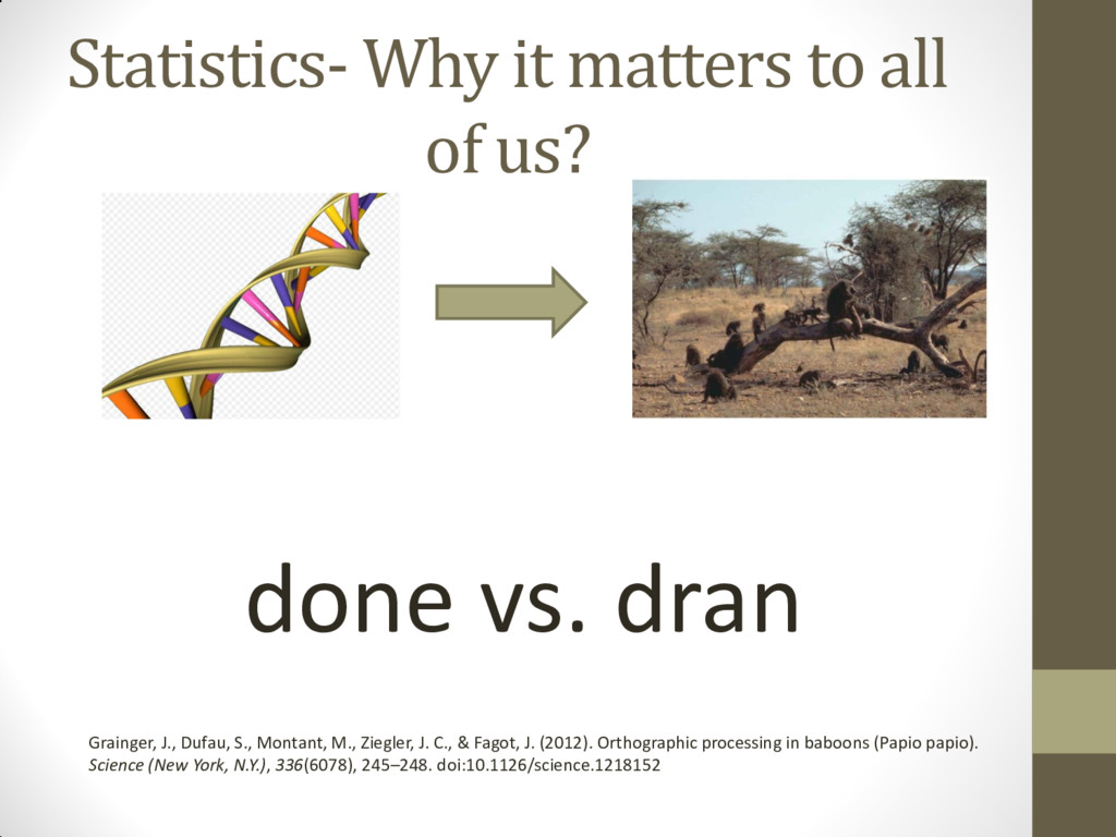
dran Grainger, J., Dufau, S., Montant, M., Ziegler, J. C., & Fagot, J. (2012). Orthographic processing in baboons (Papio papio). Science (New York, N.Y.), 336(6078), 245–248. doi:10.1126/science.1218152