Analyzing Song Structure with Spectral Clustering

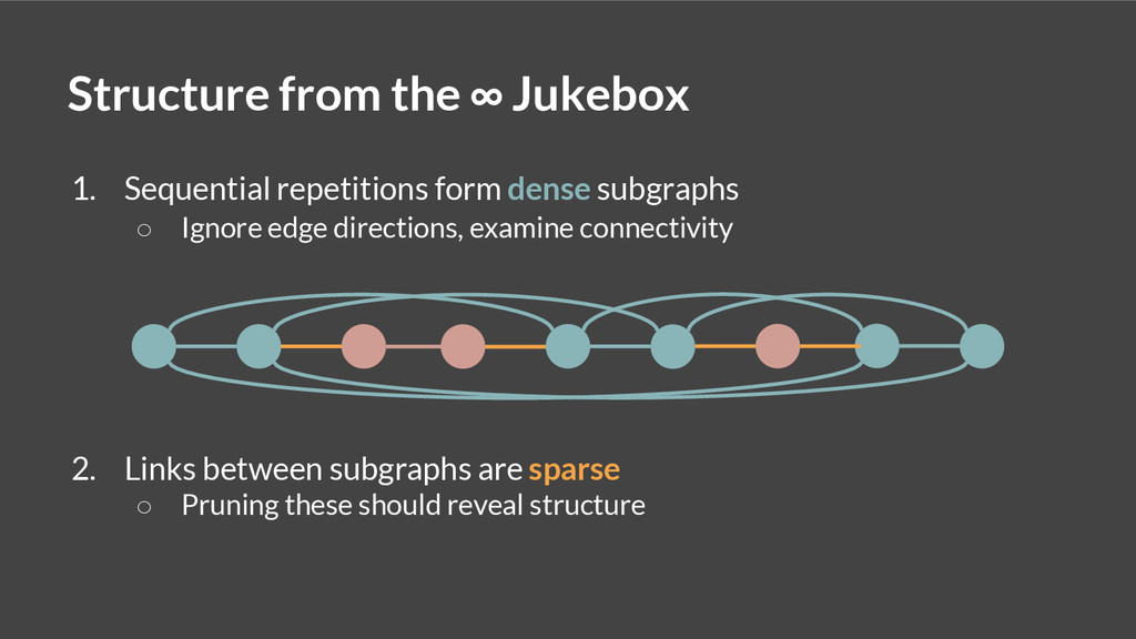
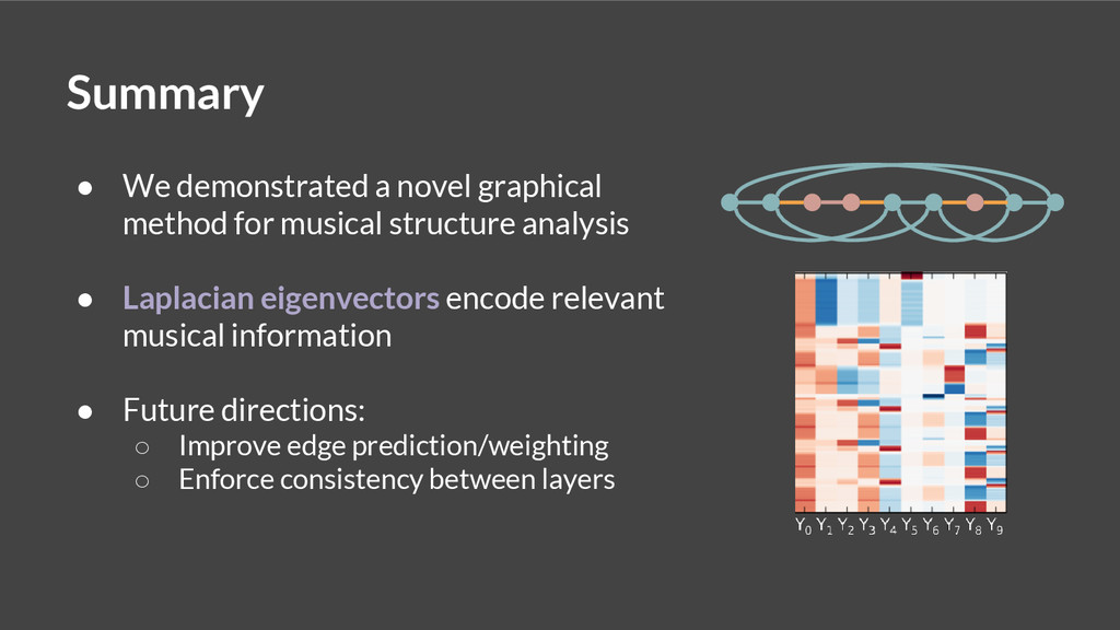
This talk describes a spectral clustering algorithm, based upon a theoretical model of the Infinite Jukebox, which can encode and expose musical structure at multiple levels of granularity.

The paper corresponding to this talk was first presented at ISMIR 2014 in Taipei.

Transcript

1. Brian McFee Dan Ellis Analyzing song structure with spectral clustering
2. Musical structure analysis 1. Detect change-points verse → chorus 2. Label repeated sections ABAC • … also representation and visualization
4. 1. Build a chain graph, each beat is a vertex 2. Connect repeated beats 3. Playback follows a random walk The Infinite Jukebox [Lamere, 2012]
5. What does this have to do with structure analysis?
6. Structure from the ∞ Jukebox 1. Sequential repetitions form dense subgraphs ◦ Ignore edge directions, examine connectivity
7. Structure from the ∞ Jukebox 1. Sequential repetitions form dense subgraphs ◦ Ignore edge directions, examine connectivity 2. Links between subgraphs are sparse ◦ Pruning these should reveal structure
8. Our strategy 1. Construct a graph over beats 2. Partition the graph to recover structure 3. Vary the partition size to expose multi-level structure
9. Building the graph [1/3]: The local graph 1. Add a vertex for each beat 2. Add local edges (i, i ± 1) 3. Weight edges by MFCC similarity 1 2 3 1 2 3 1 2 3
10. 1. Link k-nearest neighbors (in CQT space) Building the graph [2/3]: The repetition graph 3 1 2 5 6 4 8 7
11. 1. Link k-nearest neighbors (in CQT space) 2. Enhance sequences by windowed majority vote Building the graph [2/3]: The repetition graph 3 1 2 5 6 4 8 7
12. 1. Link k-nearest neighbors (in CQT space) 2. Enhance sequences by windowed majority vote Building the graph [2/3]: The repetition graph 3 1 2 5 6 4 8 7
13. 1. Link k-nearest neighbors (in CQT space) 2. Enhance sequences by windowed majority vote 3. Weight edges by feature similarity Building the graph [2/3]: The repetition graph 3 1 2 5 6 4 8 7
14. Building the graph [3/3]: The combination 1. Take a weighted combination of local and repetition A = μ *Local + (1-μ) *Repetition
15. Building the graph [3/3]: The combination 1. Take a weighted combination of local and repetition A = μ *Local + (1-μ) *Repetition 2. Optimize μ : P[Local move] ≅ P[Repetition move]
16. Building the graph [3/3]: The combination 1. Take a weighted combination of local and repetition A = μ *Local + (1-μ) *Repetition 2. Optimize μ : P[Local move] ≅ P[Repetition move] 3. μ* has a closed-form solution ∀ i: μ ∑ j Local[i,j] ≅ (1-μ) ∑ j Repetition[i,j]
17. Example: The Beatles - Come Together
18. Partitioning via spectral clustering • Affinity matrix A, degree matrix D ii = ∑ j A ij • Normalized Laplacian L = I - D-1A ◦ Bottom eigenvectors encode component membership for each beat ◦ … i.e., the regions likely to trap a random walk • Cluster the eigenvectors of L to reveal structure
19. Example: The Beatles - Come Together
20. Example: The Beatles - Come Together Low-rank reconstructions expose structure L ≅ Y[:n, :m]Y[:n, :m]T
21. Multi-level segmentation 1. Construct the n-by-n graph A 2. Compute Laplacian eigenvectors Y 3. for m in [2, 3, …] a. Partitions[m] := spectral_clustering(Y[:n, :m], n_components=m) 4. Return Partitions One discrete parameter controls complexity
22. Interactive visualization demo
23. Quantitative evaluation • Metrics: boundary detection and pairwise frame labeling ◦ Beatles_TUT (174 tracks) ◦ SALAMI small (735 tracks) and functions • Choosing the number of components ◦ Maximize label entropy with duration constraints ◦ Oracle: Best m per track, per metric (simulates interactive display) • Baseline: [Serrà, Müller, Grosche & Arcos, 2012]
24. Results: Beatles F 0.5s F 3.0s F-Pairwise Automatic m 0.312 +- 0.15 0.579 +- 0.16 0.628 +- 0.13 Oracle 0.414 +- 0.14 0.684 +- 0.13 0.694 +- 0.12 SMGA 0.293 +- 0.13 0.699 +- 0.16 0.715 +- 0.15
25. Results: SALAMI small F 0.5s F 3.0s F-Pairwise Automatic m 0.192 +- 0.11 0.344 +- 0.15 0.448 +- 0.16 Oracle 0.292 +- 0.15 0.525 +- 0.19 0.561 +- 0.16 SMGA 0.173 +- 0.08 0.518 +- 0.12 0.493 +- 0.16
26. Results: SALAMI functions F 0.5s F 3.0s F-Pairwise Automatic m 0.304 +- 0.13 0.455 +- 0.16 0.546 +- 0.14 Oracle 0.406 +- 0.13 0.579 +- 0.15 0.652 +- 0.13 SMGA 0.224 +- 0.11 0.550 +- 0.18 0.553 +- 0.15
27. Summary • We demonstrated a novel graphical method for musical structure analysis • Laplacian eigenvectors encode relevant musical information • Future directions: ◦ Improve edge prediction/weighting ◦ Enforce consistency between layers
28. Thanks! brian.mcfee@nyu.edu https://github.com/bmcfee/laplacian_segmentation https://github.com/urinieto/msaf