Adaptive Stochastic Collocation on Sparse Grids

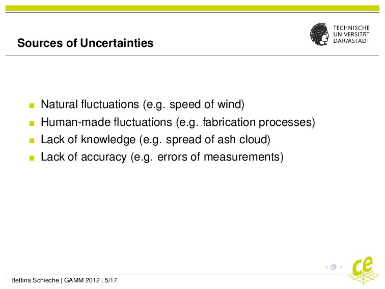
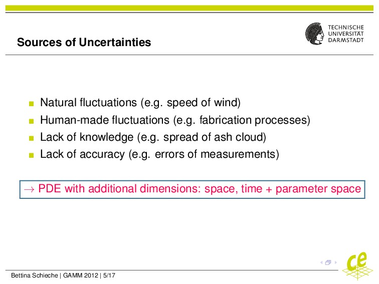
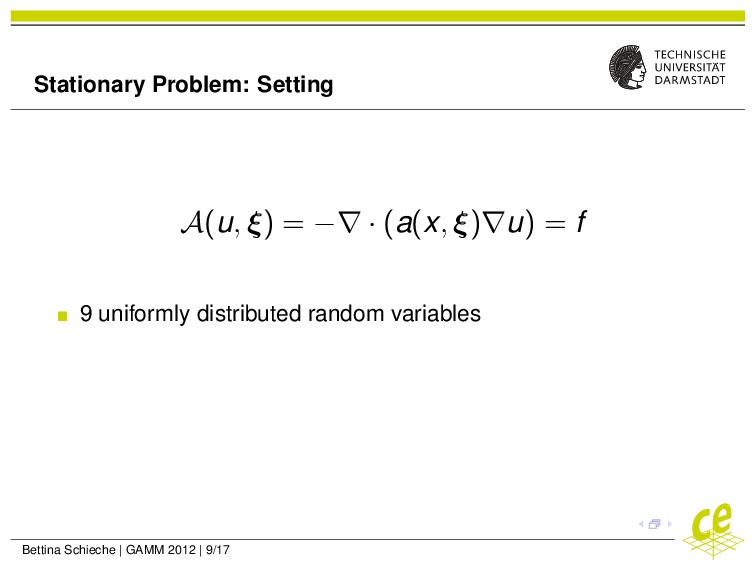
Numerical simulations become more reliable if random effects are taken into account. To this end, the describing parameters can be expressed by random variables or random fields, which leads to partial differential equations (PDEs) with random parameters.
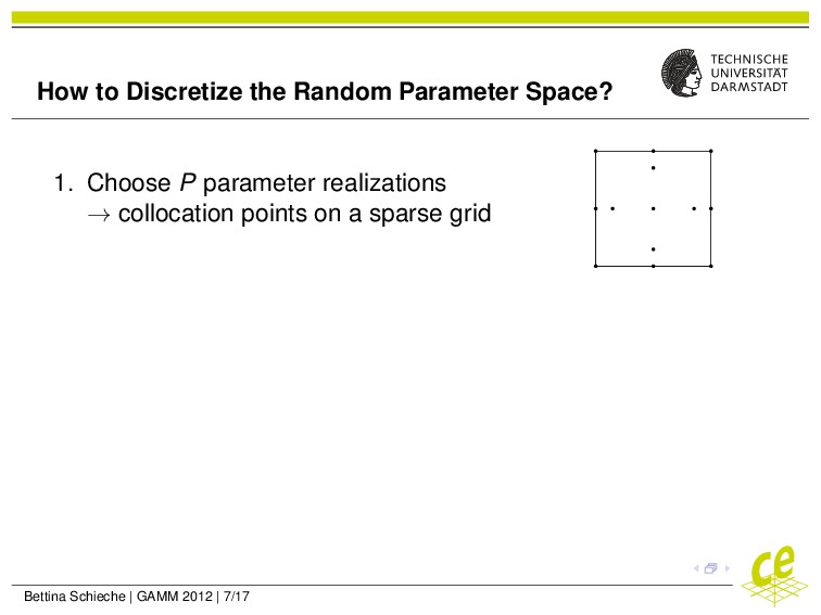
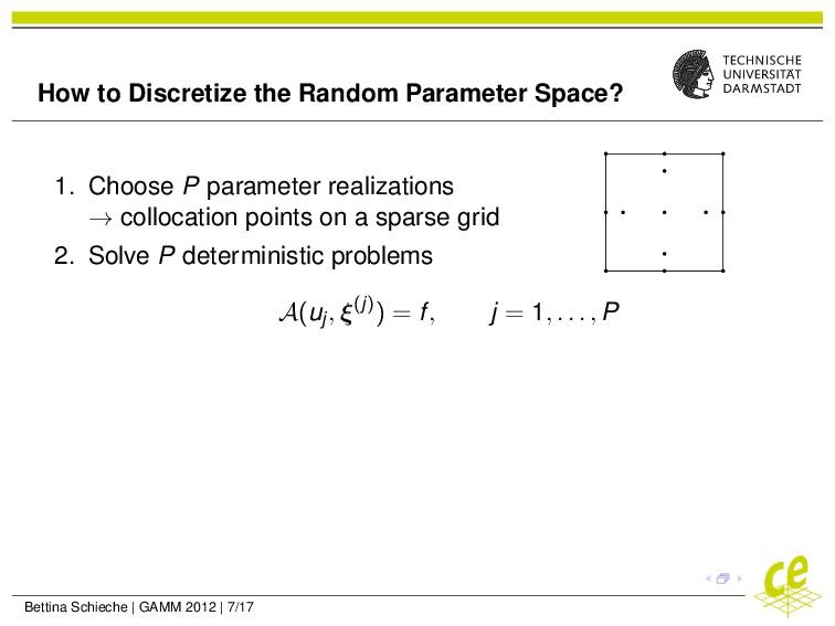
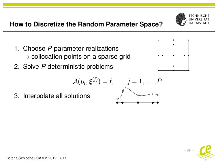
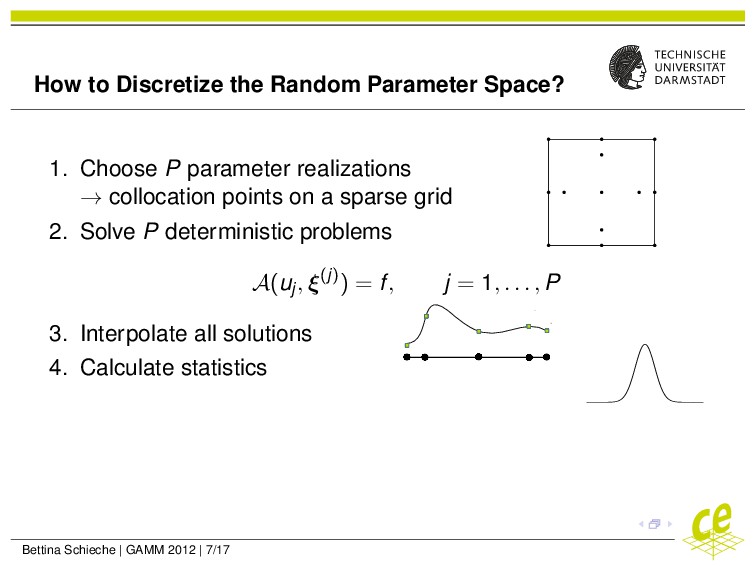
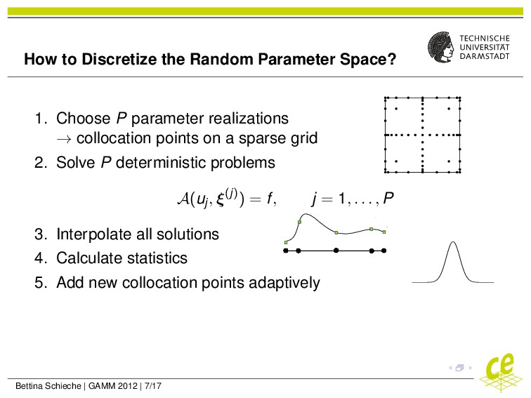
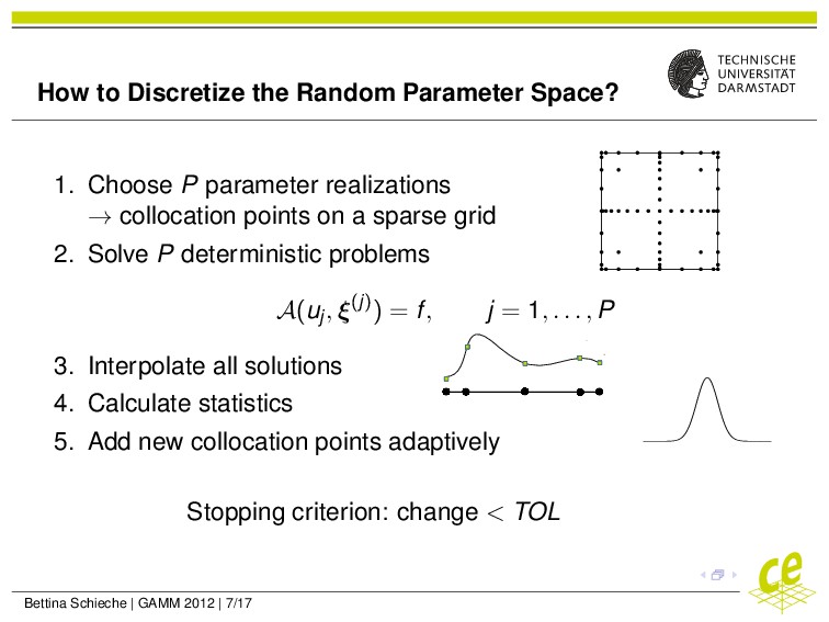
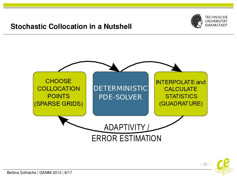
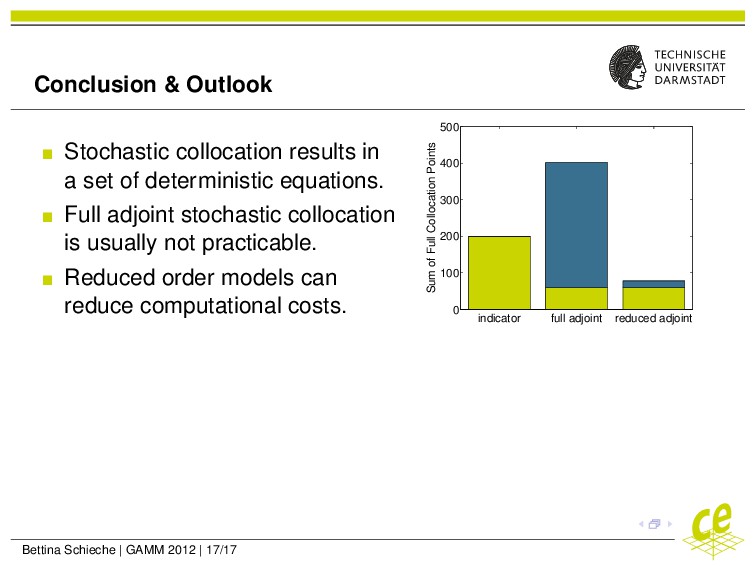
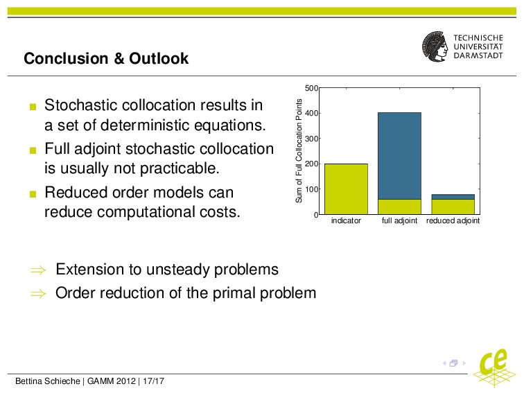
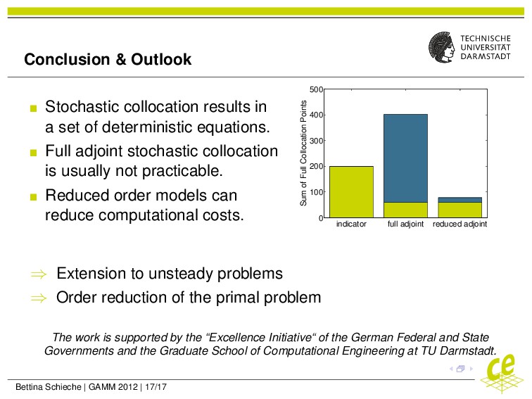
Common numerical methods to solve such problems are spectral methods of Galerkin type and stochastic collocation on sparse grids. We focus on stochastic collocation, because it decouples the random PDE into a set of deterministic equations that can be solved in parallel.
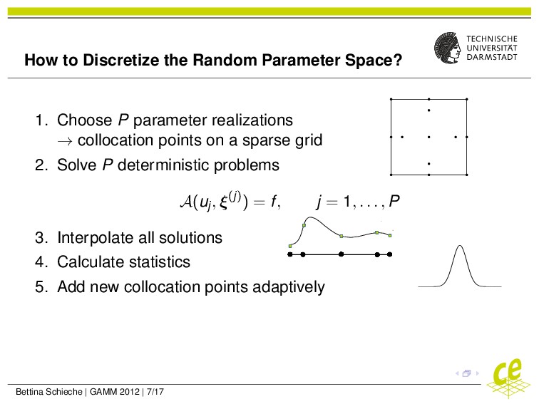
In order to keep the computational costs at a moderate level, it is inevitable to place the collocation points adaptively. Therefore, error estimates are required. For spectral methods, adjoint a posteriori error analysis has been proposed in.
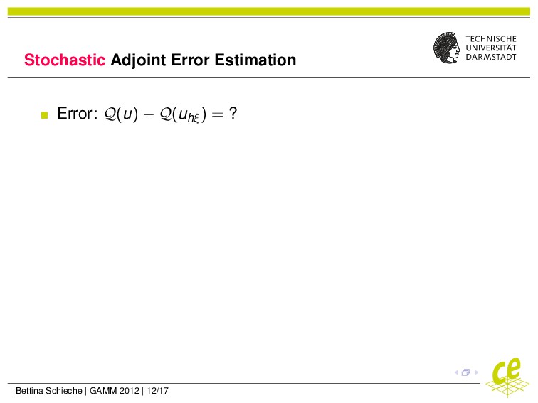
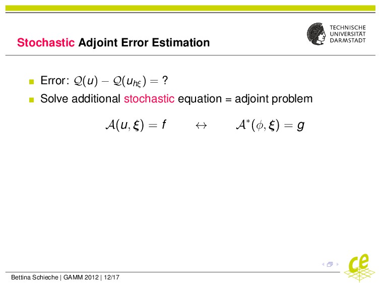
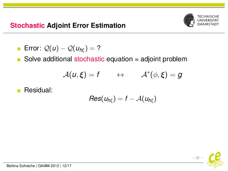
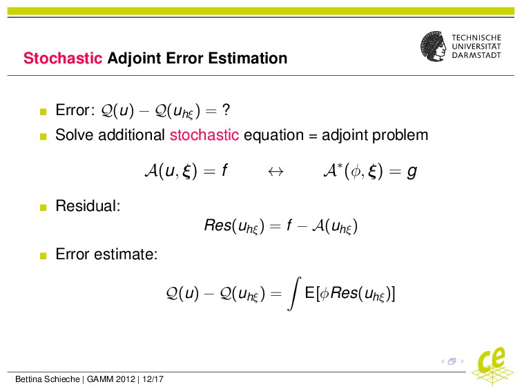
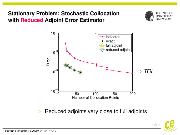
We want to combine stochastic collocation with an adjoint approach in order to estimate the error of some stochastic quantity, such as the mean or variance of a solution functional. Thereby, our goal is to develop appropriate error estimates that require less computational effort then the solution itself.

Transcript

1. Adaptive Stochastic Collocation on Sparse Grids Bettina Schieche Graduate School of Computational Engineering Numerical Analysis and Scientific Computing Technische Universität Darmstadt Numerical Analysis GAMM 2012 Darmstadt, March 29, 2012 www.graduate-school-ce.de March 29, 2012
2. Outline Motivation for PDEs with Random Parameters Adaptive Stochastic Collocation Method Adjoint Error Estimation Bettina Schieche | GAMM 2012 | 2/17
3. Overview Motivation for PDEs with Random Parameters Adaptive Stochastic Collocation Method Adjoint Error Estimation Bettina Schieche | GAMM 2012 | 3/17
4. General Setting: Arbitrary PDE Describing parameters: Boundary and initial conditions Material properties Forcing terms / source terms Topology (geometry of the system) Bettina Schieche | GAMM 2012 | 4/17
5. Sources of Uncertainties Natural fluctuations (e.g. speed of wind) Human-made fluctuations (e.g. fabrication processes) Lack of knowledge (e.g. spread of ash cloud) Lack of accuracy (e.g. errors of measurements) Bettina Schieche | GAMM 2012 | 5/17
6. Sources of Uncertainties Natural fluctuations (e.g. speed of wind) Human-made fluctuations (e.g. fabrication processes) Lack of knowledge (e.g. spread of ash cloud) Lack of accuracy (e.g. errors of measurements) → PDE with additional dimensions: space, time + parameter space Bettina Schieche | GAMM 2012 | 5/17
7. Overview Motivation for PDEs with Random Parameters Adaptive Stochastic Collocation Method Adjoint Error Estimation Bettina Schieche | GAMM 2012 | 6/17
8. How to Discretize the Random Parameter Space? 1. Choose P parameter realizations → collocation points on a sparse grid Bettina Schieche | GAMM 2012 | 7/17
9. How to Discretize the Random Parameter Space? 1. Choose P parameter realizations → collocation points on a sparse grid 2. Solve P deterministic problems A(uj, ξ(j)) = f, j = 1, . . . , P Bettina Schieche | GAMM 2012 | 7/17
10. How to Discretize the Random Parameter Space? 1. Choose P parameter realizations → collocation points on a sparse grid 2. Solve P deterministic problems A(uj, ξ(j)) = f, j = 1, . . . , P 3. Interpolate all solutions Bettina Schieche | GAMM 2012 | 7/17
11. How to Discretize the Random Parameter Space? 1. Choose P parameter realizations → collocation points on a sparse grid 2. Solve P deterministic problems A(uj, ξ(j)) = f, j = 1, . . . , P 3. Interpolate all solutions 4. Calculate statistics Bettina Schieche | GAMM 2012 | 7/17
12. How to Discretize the Random Parameter Space? 1. Choose P parameter realizations → collocation points on a sparse grid 2. Solve P deterministic problems A(uj, ξ(j)) = f, j = 1, . . . , P 3. Interpolate all solutions 4. Calculate statistics 5. Add new collocation points adaptively Bettina Schieche | GAMM 2012 | 7/17
13. How to Discretize the Random Parameter Space? 1. Choose P parameter realizations → collocation points on a sparse grid 2. Solve P deterministic problems A(uj, ξ(j)) = f, j = 1, . . . , P 3. Interpolate all solutions 4. Calculate statistics 5. Add new collocation points adaptively Bettina Schieche | GAMM 2012 | 7/17
14. How to Discretize the Random Parameter Space? 1. Choose P parameter realizations → collocation points on a sparse grid 2. Solve P deterministic problems A(uj, ξ(j)) = f, j = 1, . . . , P 3. Interpolate all solutions 4. Calculate statistics 5. Add new collocation points adaptively Bettina Schieche | GAMM 2012 | 7/17
15. How to Discretize the Random Parameter Space? 1. Choose P parameter realizations → collocation points on a sparse grid 2. Solve P deterministic problems A(uj, ξ(j)) = f, j = 1, . . . , P 3. Interpolate all solutions 4. Calculate statistics 5. Add new collocation points adaptively Stopping criterion: change < TOL Bettina Schieche | GAMM 2012 | 7/17
16. Stochastic Collocation in a Nutshell DETERMINISTIC PDE-SOLVER CHOOSE COLLOCATION POINTS (SPARSE GRIDS) INTERPOLATE and CALCULATE STATISTICS (QUADRATURE) ADAPTIVITY / ERROR ESTIMATION Bettina Schieche | GAMM 2012 | 8/17
17. Stationary Problem: Setting A(u, ξ) = −∇ · (a(x, ξ)∇u) = f 9 uniformly distributed random variables Bettina Schieche | GAMM 2012 | 9/17
18. Stationary Problem: Setting A(u, ξ) = −∇ · (a(x, ξ)∇u) = f 9 uniformly distributed random variables Quantity of interest: Q(u) = E[u] Bettina Schieche | GAMM 2012 | 9/17
19. Stationary Problem: Setting A(u, ξ) = −∇ · (a(x, ξ)∇u) = f 9 uniformly distributed random variables Quantity of interest: Q(u) = E[u] Stochastic collocation → uhξ Bettina Schieche | GAMM 2012 | 9/17
20. Stationary Problem: Setting A(u, ξ) = −∇ · (a(x, ξ)∇u) = f 9 uniformly distributed random variables Quantity of interest: Q(u) = E[u] Stochastic collocation → uhξ Aim: Q(u) − Q(uhξ ) ! < TOL = 10−3 Bettina Schieche | GAMM 2012 | 9/17
21. Stationary Problem: Results 0 50 100 150 200 10−4 10−3 10−2 10−1 Number of Collocation Points Error indicator exact ⇒ Much more collocation points than necessary → TOL Bettina Schieche | GAMM 2012 | 10/17
22. Overview Motivation for PDEs with Random Parameters Adaptive Stochastic Collocation Method Adjoint Error Estimation Bettina Schieche | GAMM 2012 | 11/17
23. Stochastic Adjoint Error Estimation Error: Q(u) − Q(uhξ ) = ? Bettina Schieche | GAMM 2012 | 12/17
24. Stochastic Adjoint Error Estimation Error: Q(u) − Q(uhξ ) = ? Solve additional stochastic equation = adjoint problem A(u, ξ) = f ↔ A∗(φ, ξ) = g Bettina Schieche | GAMM 2012 | 12/17
25. Stochastic Adjoint Error Estimation Error: Q(u) − Q(uhξ ) = ? Solve additional stochastic equation = adjoint problem A(u, ξ) = f ↔ A∗(φ, ξ) = g Residual: Res(uhξ ) = f − A(uhξ ) Bettina Schieche | GAMM 2012 | 12/17
26. Stochastic Adjoint Error Estimation Error: Q(u) − Q(uhξ ) = ? Solve additional stochastic equation = adjoint problem A(u, ξ) = f ↔ A∗(φ, ξ) = g Residual: Res(uhξ ) = f − A(uhξ ) Error estimate: Q(u) − Q(uhξ ) = E[φRes(uhξ )] Bettina Schieche | GAMM 2012 | 12/17
27. Stationary Problem: Stochastic Adjoint Error Analysis Error splitting: Q(u) − Q(uhξ ) joint error = Q(u) − Q(uξ) stochastic error + Q(uξ) − Q(uhξ ) deterministic error Bettina Schieche | GAMM 2012 | 13/17
28. Stationary Problem: Stochastic Adjoint Error Analysis Error splitting: Q(u) − Q(uhξ ) joint error = Q(u) − Q(uξ) stochastic error + Q(uξ) − Q(uhξ ) deterministic error 0 200 400 600 800 0 0.2 0.4 0.6 0.8 1 number of adjoint collocation points estimate / exact error deterministic error joint error stochastic error ⇒ Much effort to capture stochastic error ⇒ Few effort to capture determinitic error Bettina Schieche | GAMM 2012 | 13/17
29. Stationary Problem: Stochastic Collocation with Full Adjoint Error Estimates 0 50 100 150 200 10−4 10−3 10−2 10−1 Number of Collocation Points Error indicator exact full adjoint ⇒ Error estimates very accurate ⇒ Drawback: > 300 adjoint collocation points → TOL Bettina Schieche | GAMM 2012 | 14/17
30. Idea: Order Reduction of Adjoint Problem 1. One iteration of stochastic collocation: A(ξ(j))Uj = F 2. Adjoint solutions in these collocation points: A∗(ξ(j))Φj = G 3. Snapshot matrix S = (Φ1, · · · , ΦP) 4. Singular value decomposition of S → reduced basis ϕ 5. Galerkin projection onto ϕ: A∗ R (ξ)ΦR(ξ) = GR, dim(A∗ R ) dim(A∗) (1) 6. Evaluation of (1) in many adjoint collocation points Bettina Schieche | GAMM 2012 | 15/17
31. Stationary Problem: Stochastic Collocation with Reduced Adjoint Error Estimator 0 50 100 150 200 10−4 10−3 10−2 10−1 Number of Collocation Points Error indicator exact full adjoint reduced adjoint ⇒ Reduced adjoints very close to full adjoints → TOL Bettina Schieche | GAMM 2012 | 16/17
32. Conclusion & Outlook Stochastic collocation results in a set of deterministic equations. Full adjoint stochastic collocation is usually not practicable. Reduced order models can reduce computational costs. indicator full adjoint reduced adjoint 0 100 200 300 400 500 Sum of Full Collocation Points Bettina Schieche | GAMM 2012 | 17/17
33. Conclusion & Outlook Stochastic collocation results in a set of deterministic equations. Full adjoint stochastic collocation is usually not practicable. Reduced order models can reduce computational costs. indicator full adjoint reduced adjoint 0 100 200 300 400 500 Sum of Full Collocation Points ⇒ Extension to unsteady problems ⇒ Order reduction of the primal problem Bettina Schieche | GAMM 2012 | 17/17
34. Conclusion & Outlook Stochastic collocation results in a set of deterministic equations. Full adjoint stochastic collocation is usually not practicable. Reduced order models can reduce computational costs. indicator full adjoint reduced adjoint 0 100 200 300 400 500 Sum of Full Collocation Points ⇒ Extension to unsteady problems ⇒ Order reduction of the primal problem The work is supported by the “Excellence Initiative“ of the German Federal and State Governments and the Graduate School of Computational Engineering at TU Darmstadt. Bettina Schieche | GAMM 2012 | 17/17