Adjoint Error Estimation for Stochastic Collocation Methods

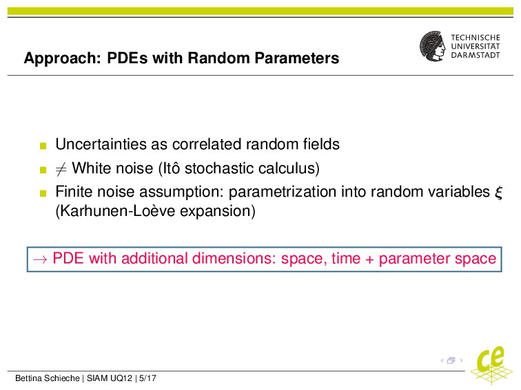
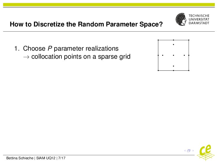
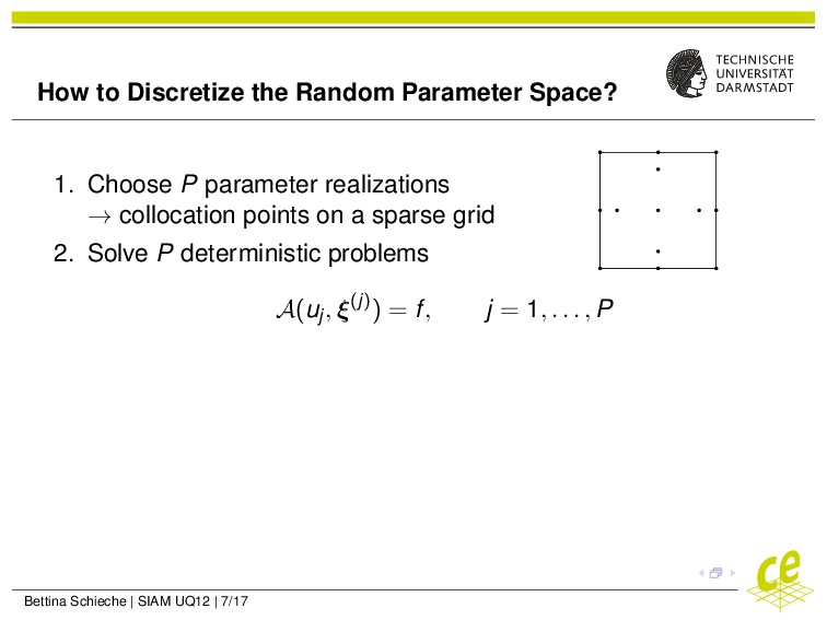
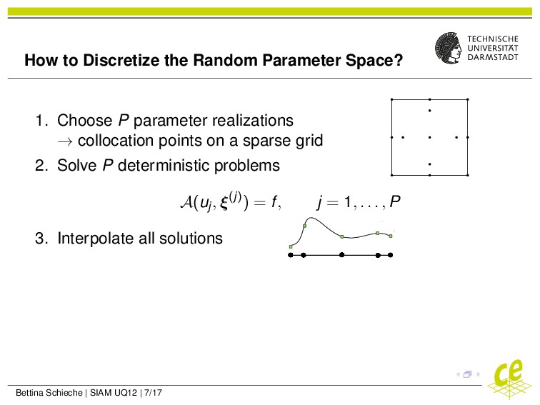
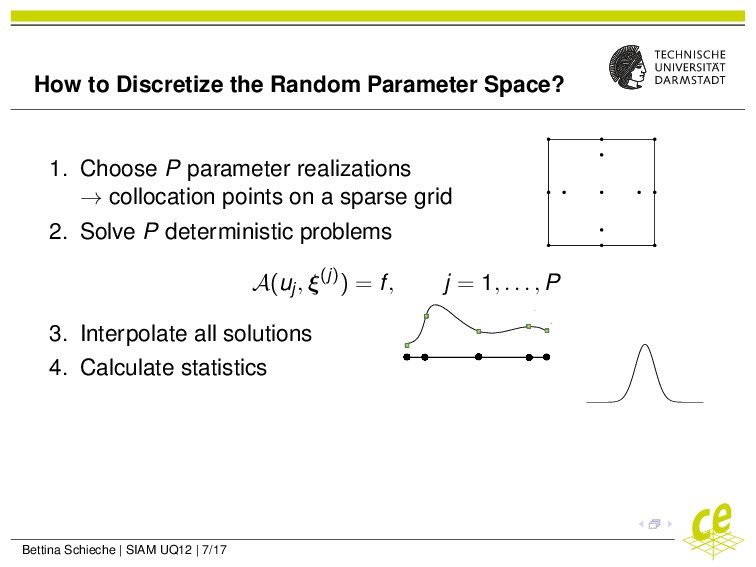
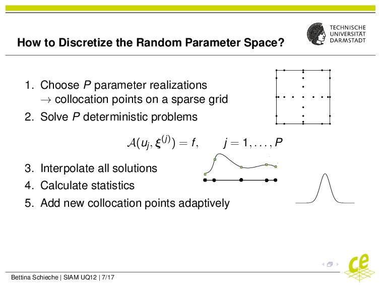
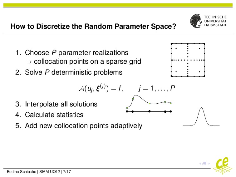
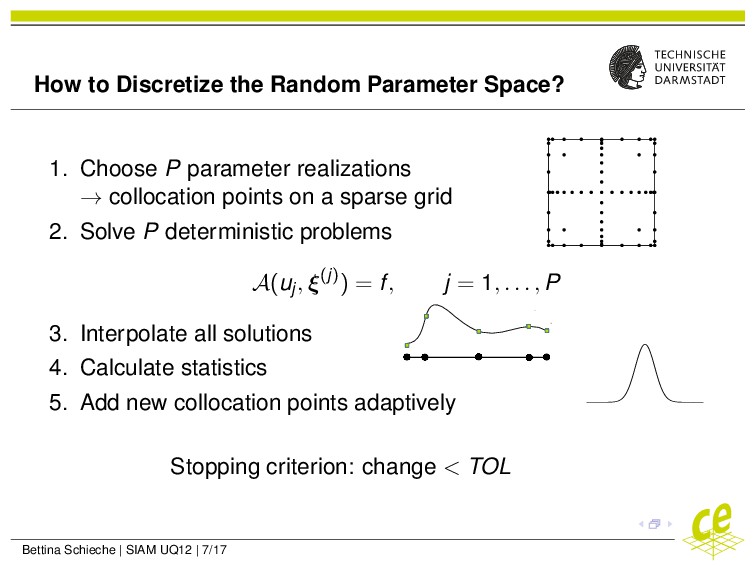
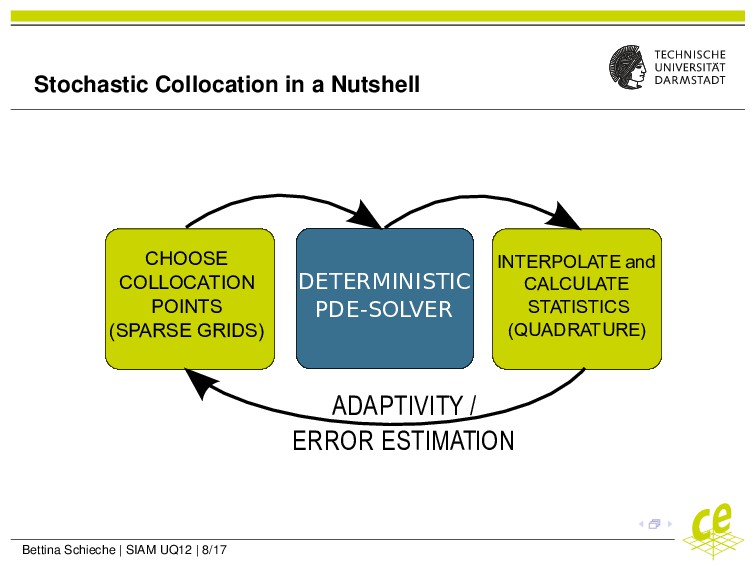
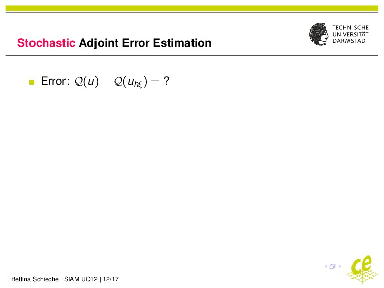
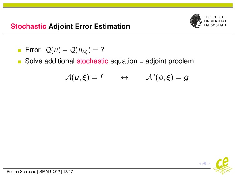
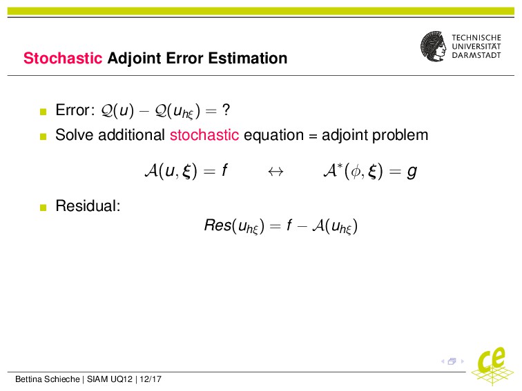
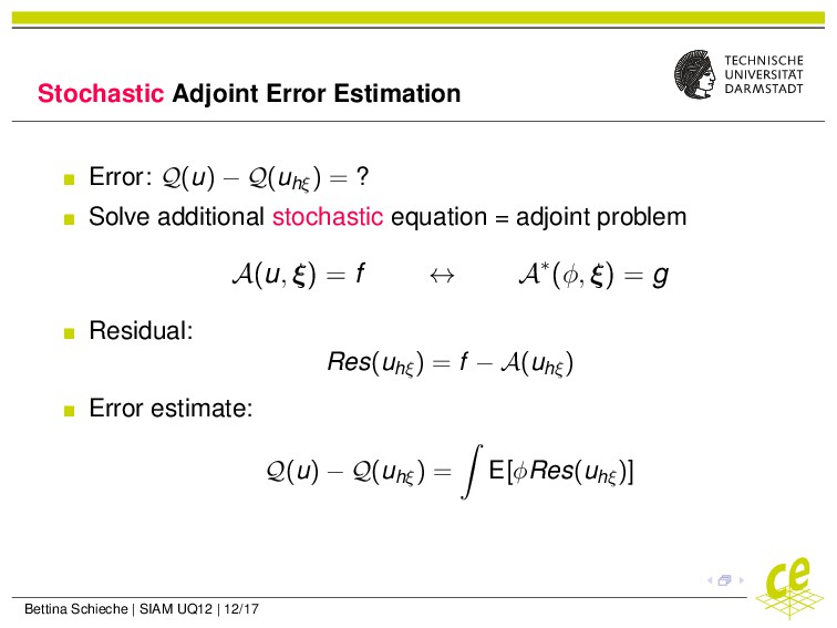
We use anisotropic, stochastic collocation on sparse grids for solving partial differential equations (PDEs) with random parameters. Our aim is to combine the method with an adjoint approach in order to estimate and control the error of some stochastic quantity, such as the mean or variance of a solution functional. Therefore, our goal is to provide appropriate error estimates that require less computational effort then the collocation procedure itself.

Transcript

1. Adjoint Error Estimation for Stochastic Collocation Methods Bettina Schieche Graduate School of Computational Engineering Numerical Analysis and Scientific Computing Technische Universität Darmstadt Numerical Analysis SIAM Conference on Uncertainty Quantification Raleigh, North Carolina USA, April 2, 2012 www.graduate-school-ce.de April 2, 2012
2. Outline Setting: PDEs with Random Parameters Adaptive Stochastic Collocation Method Adjoint Error Estimation Bettina Schieche | SIAM UQ12 | 2/17
3. Overview Setting: PDEs with Random Parameters Adaptive Stochastic Collocation Method Adjoint Error Estimation Bettina Schieche | SIAM UQ12 | 3/17
4. General Setting: PDE with Uncertainties Uncertainties might arise in: Boundary and initial conditions Material properties Forcing terms / source terms Topology (geometry of the system) Bettina Schieche | SIAM UQ12 | 4/17
5. Approach: PDEs with Random Parameters Uncertainties as correlated random fields = White noise (Itô stochastic calculus) Finite noise assumption: parametrization into random variables ξ (Karhunen-Loève expansion) Bettina Schieche | SIAM UQ12 | 5/17
6. Approach: PDEs with Random Parameters Uncertainties as correlated random fields = White noise (Itô stochastic calculus) Finite noise assumption: parametrization into random variables ξ (Karhunen-Loève expansion) → PDE with additional dimensions: space, time + parameter space Bettina Schieche | SIAM UQ12 | 5/17
7. Overview Setting: PDEs with Random Parameters Adaptive Stochastic Collocation Method Adjoint Error Estimation Bettina Schieche | SIAM UQ12 | 6/17
8. How to Discretize the Random Parameter Space? 1. Choose P parameter realizations → collocation points on a sparse grid Bettina Schieche | SIAM UQ12 | 7/17
9. How to Discretize the Random Parameter Space? 1. Choose P parameter realizations → collocation points on a sparse grid 2. Solve P deterministic problems A(uj, ξ(j)) = f, j = 1, . . . , P Bettina Schieche | SIAM UQ12 | 7/17
10. How to Discretize the Random Parameter Space? 1. Choose P parameter realizations → collocation points on a sparse grid 2. Solve P deterministic problems A(uj, ξ(j)) = f, j = 1, . . . , P 3. Interpolate all solutions Bettina Schieche | SIAM UQ12 | 7/17
11. How to Discretize the Random Parameter Space? 1. Choose P parameter realizations → collocation points on a sparse grid 2. Solve P deterministic problems A(uj, ξ(j)) = f, j = 1, . . . , P 3. Interpolate all solutions 4. Calculate statistics Bettina Schieche | SIAM UQ12 | 7/17
12. How to Discretize the Random Parameter Space? 1. Choose P parameter realizations → collocation points on a sparse grid 2. Solve P deterministic problems A(uj, ξ(j)) = f, j = 1, . . . , P 3. Interpolate all solutions 4. Calculate statistics 5. Add new collocation points adaptively Bettina Schieche | SIAM UQ12 | 7/17
13. How to Discretize the Random Parameter Space? 1. Choose P parameter realizations → collocation points on a sparse grid 2. Solve P deterministic problems A(uj, ξ(j)) = f, j = 1, . . . , P 3. Interpolate all solutions 4. Calculate statistics 5. Add new collocation points adaptively Bettina Schieche | SIAM UQ12 | 7/17
14. How to Discretize the Random Parameter Space? 1. Choose P parameter realizations → collocation points on a sparse grid 2. Solve P deterministic problems A(uj, ξ(j)) = f, j = 1, . . . , P 3. Interpolate all solutions 4. Calculate statistics 5. Add new collocation points adaptively Bettina Schieche | SIAM UQ12 | 7/17
15. How to Discretize the Random Parameter Space? 1. Choose P parameter realizations → collocation points on a sparse grid 2. Solve P deterministic problems A(uj, ξ(j)) = f, j = 1, . . . , P 3. Interpolate all solutions 4. Calculate statistics 5. Add new collocation points adaptively Stopping criterion: change < TOL Bettina Schieche | SIAM UQ12 | 7/17
16. Stochastic Collocation in a Nutshell DETERMINISTIC PDE-SOLVER CHOOSE COLLOCATION POINTS (SPARSE GRIDS) INTERPOLATE and CALCULATE STATISTICS (QUADRATURE) ADAPTIVITY / ERROR ESTIMATION Bettina Schieche | SIAM UQ12 | 8/17
17. Stationary Problem: Setting A(u, ξ) = −∇ · (a(x, ξ)∇u) = f 9 uniformly distributed random variables Bettina Schieche | SIAM UQ12 | 9/17
18. Stationary Problem: Setting A(u, ξ) = −∇ · (a(x, ξ)∇u) = f 9 uniformly distributed random variables Quantity of interest: Q(u) = E[u] Bettina Schieche | SIAM UQ12 | 9/17
19. Stationary Problem: Setting A(u, ξ) = −∇ · (a(x, ξ)∇u) = f 9 uniformly distributed random variables Quantity of interest: Q(u) = E[u] Stochastic collocation → uhξ Bettina Schieche | SIAM UQ12 | 9/17
20. Stationary Problem: Setting A(u, ξ) = −∇ · (a(x, ξ)∇u) = f 9 uniformly distributed random variables Quantity of interest: Q(u) = E[u] Stochastic collocation → uhξ Aim: Q(u) − Q(uhξ ) ! < TOL = 10−3 Bettina Schieche | SIAM UQ12 | 9/17
21. Stationary Problem: Results 0 5 10 15 10−4 10−3 10−2 10−1 P = 199 P = 59 Iterations Error indicator exact ⇒ Much more collocation points than necessary → TOL Bettina Schieche | SIAM UQ12 | 10/17
22. Overview Setting: PDEs with Random Parameters Adaptive Stochastic Collocation Method Adjoint Error Estimation Bettina Schieche | SIAM UQ12 | 11/17
23. Stochastic Adjoint Error Estimation Error: Q(u) − Q(uhξ ) = ? Bettina Schieche | SIAM UQ12 | 12/17
24. Stochastic Adjoint Error Estimation Error: Q(u) − Q(uhξ ) = ? Solve additional stochastic equation = adjoint problem A(u, ξ) = f ↔ A∗(φ, ξ) = g Bettina Schieche | SIAM UQ12 | 12/17
25. Stochastic Adjoint Error Estimation Error: Q(u) − Q(uhξ ) = ? Solve additional stochastic equation = adjoint problem A(u, ξ) = f ↔ A∗(φ, ξ) = g Residual: Res(uhξ ) = f − A(uhξ ) Bettina Schieche | SIAM UQ12 | 12/17
26. Stochastic Adjoint Error Estimation Error: Q(u) − Q(uhξ ) = ? Solve additional stochastic equation = adjoint problem A(u, ξ) = f ↔ A∗(φ, ξ) = g Residual: Res(uhξ ) = f − A(uhξ ) Error estimate: Q(u) − Q(uhξ ) = E[φRes(uhξ )] Bettina Schieche | SIAM UQ12 | 12/17
27. Stationary Problem: Stochastic Adjoint Error Analysis Error splitting: Q(u) − Q(uhξ ) joint error = Q(u) − Q(uξ) stochastic error + Q(uξ) − Q(uhξ ) deterministic error Bettina Schieche | SIAM UQ12 | 13/17
28. Stationary Problem: Stochastic Adjoint Error Analysis Error splitting: Q(u) − Q(uhξ ) joint error = Q(u) − Q(uξ) stochastic error + Q(uξ) − Q(uhξ ) deterministic error 0 200 400 600 800 0 0.2 0.4 0.6 0.8 1 number of adjoint collocation points estimate / exact error deterministic error joint error stochastic error ⇒ Much effort to capture stochastic error ⇒ Few effort to capture determinitic error Bettina Schieche | SIAM UQ12 | 13/17
29. Stationary Problem: Stochastic Collocation with Full Adjoint Error Estimates 0 5 10 15 10−4 10−3 10−2 10−1 P = 199 P = 59 Iterations Error indicator exact full adjoint ⇒ Error estimates very accurate ⇒ Drawback: > 300 adjoint collocation points → TOL Bettina Schieche | SIAM UQ12 | 14/17
30. Idea: Order Reduction of Adjoint Problem 1. One iteration of stochastic collocation: A(ξ(j))Uj = F 2. Adjoint solutions in these collocation points: A∗(ξ(j))Φj = G 3. Snapshot matrix S = (Φ1, · · · , ΦP) 4. Singular value decomposition of S → reduced basis ϕ 5. Galerkin projection onto ϕ: A∗ R (ξ)ΦR(ξ) = GR, dim(A∗ R ) dim(A∗) (1) 6. Evaluation of (1) in many adjoint collocation points Bettina Schieche | SIAM UQ12 | 15/17
31. Stationary Problem: Stochastic Collocation with Reduced Adjoint Error Estimator 0 5 10 15 10−4 10−3 10−2 10−1 P = 199 P = 59 Iterations Error indicator exact full adjoint reduced adjoint ⇒ Reduced adjoints very close to full adjoints → TOL Bettina Schieche | SIAM UQ12 | 16/17
32. Conclusion & Outlook Stochastic collocation results in a set of deterministic equations. Full adjoint stochastic collocation is usually not practicable. Reduced order models can reduce computational costs. indicator full adjoint reduced adjoint 0 100 200 300 400 500 Sum of Full Collocation Points Bettina Schieche | SIAM UQ12 | 17/17
33. Conclusion & Outlook Stochastic collocation results in a set of deterministic equations. Full adjoint stochastic collocation is usually not practicable. Reduced order models can reduce computational costs. indicator full adjoint reduced adjoint 0 100 200 300 400 500 Sum of Full Collocation Points ⇒ Extension to unsteady problems ⇒ Order reduction of the primal problem Bettina Schieche | SIAM UQ12 | 17/17
34. Conclusion & Outlook Stochastic collocation results in a set of deterministic equations. Full adjoint stochastic collocation is usually not practicable. Reduced order models can reduce computational costs. indicator full adjoint reduced adjoint 0 100 200 300 400 500 Sum of Full Collocation Points ⇒ Extension to unsteady problems ⇒ Order reduction of the primal problem The work is supported by the “Excellence Initiative“ of the German Federal and State Governments and the Graduate School of Computational Engineering at TU Darmstadt. Bettina Schieche | SIAM UQ12 | 17/17