Analysis and Application of PDEs with Random Parameters

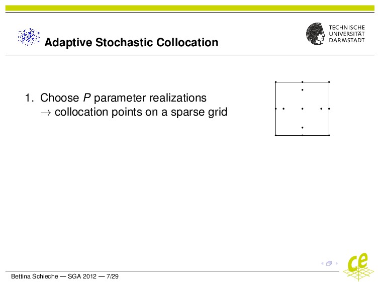
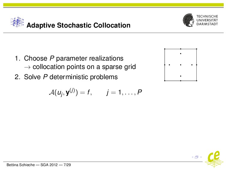
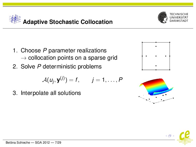
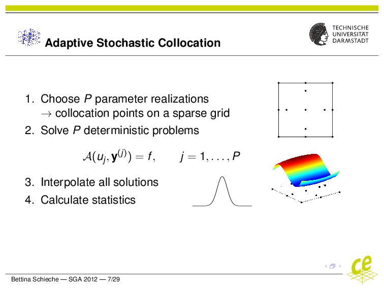
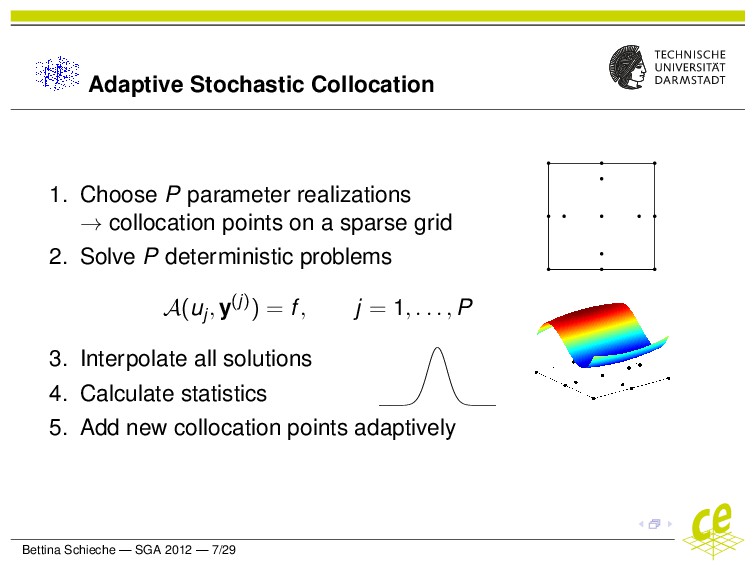
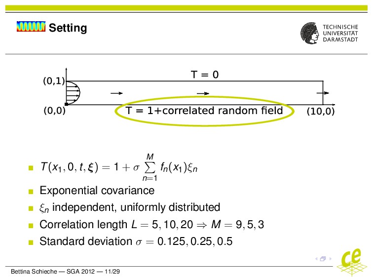
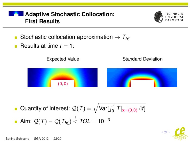
Uncertain input data for partial differential equations (PDEs) are often reason- ably described by a set of independent random variables. To discretize the re- sulting parameter space, Monte Carlo simulations, spectral methods of Galerkin type, or stochastic collocation on sparse grids can be used. We focus on the latter, because it decouples the problem into a set of deterministic equations, while being able to achieve high convergence rates.
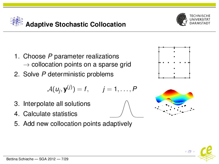
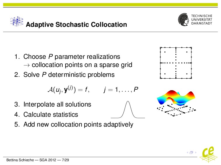
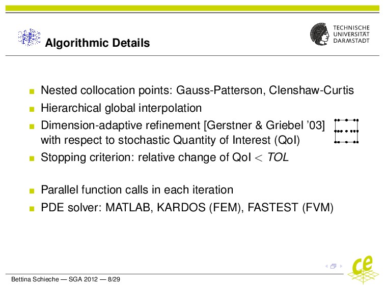
We adaptively choose the collocation points on anisotropic sparse grids based on Gauss-Patterson quadrature nodes and Smolyak’s algorithm. Moreover, we describe the random solution field in terms of hierarchical Lagrange polynomials. The hierarchical surpluses can naturally be used as error indicators, because they contain the amount of change in the solution with respect to new collocation points. The algorithm terminates when this change falls under a given tolerance.
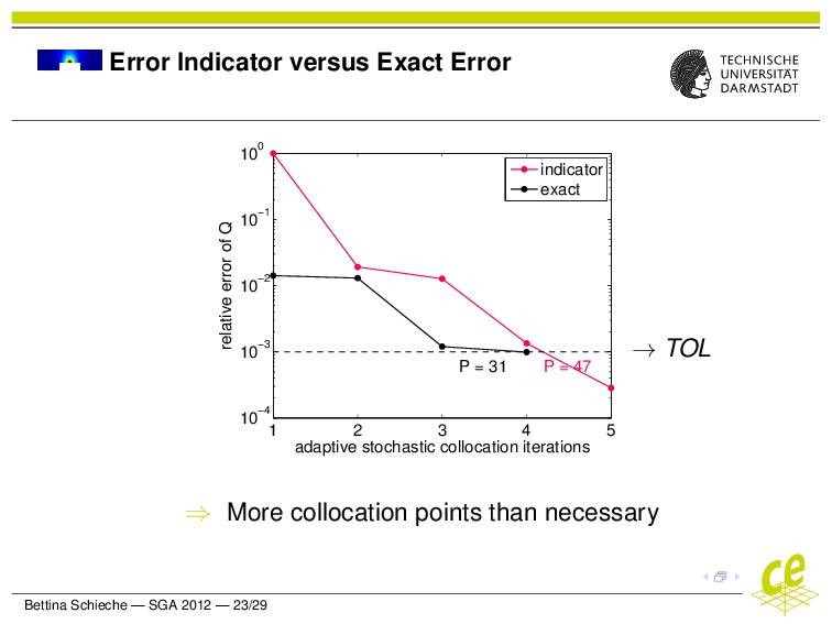
Our experience includes elliptic, parabolic, and various flow problems with random parameters, where we have used up to 17 random dimensions so far. We observe that adaptive stochastic collocation performs quite well for all examples, but overestimates the interpolation error in some cases, leading to more collocation points than actually necessary. One reason for that is that the algorithm can only terminate properly, when the stochastic tolerance is not chosen smaller than deterministic discretization errors.
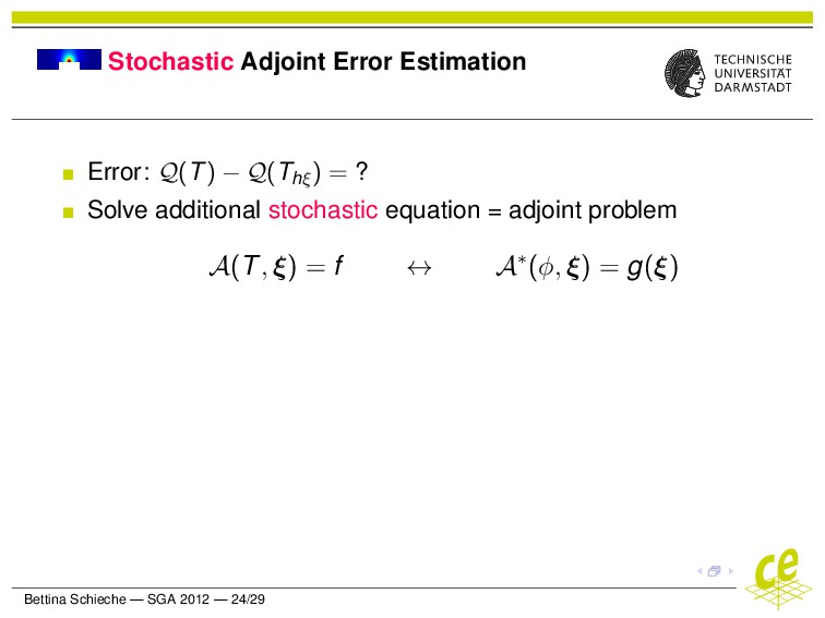
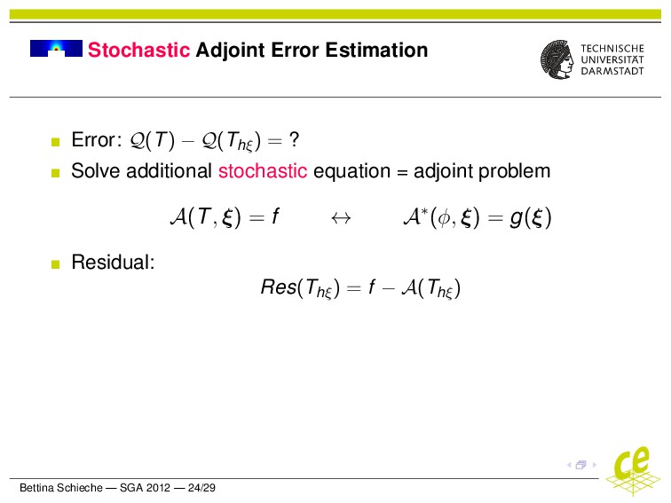
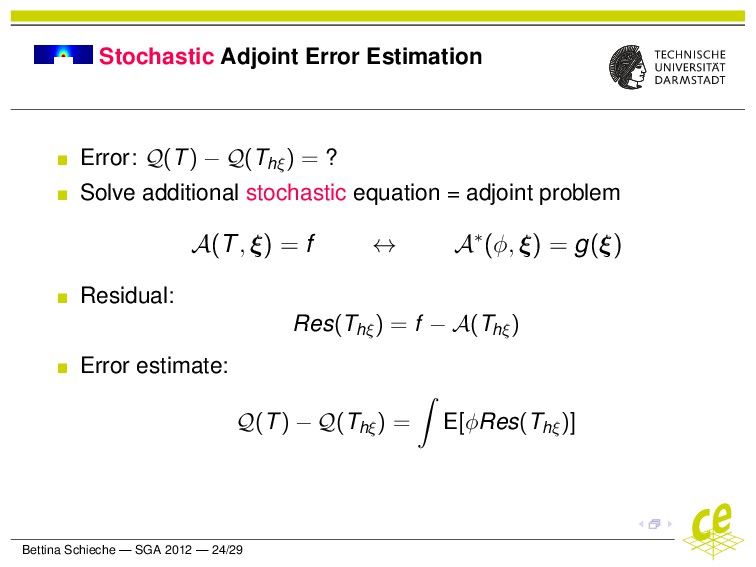
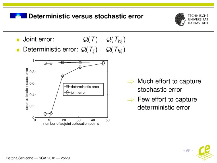
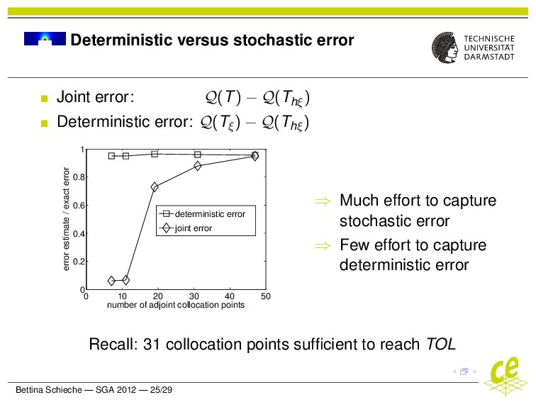
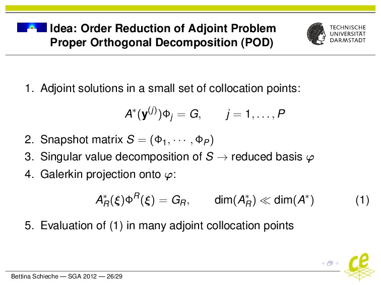
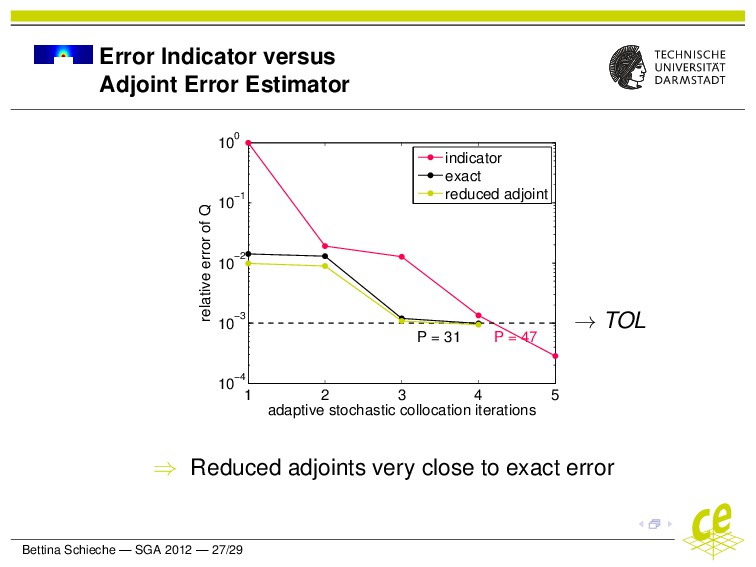
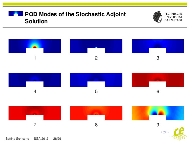
Our aim is to analyze and detect deterministic and stochastic errors. To this end, we use an adjoint approach to obtain more accurate error estimates than given by the error indicators. What we see is that adjoint stochastic collocation needs a few collocation points to capture deterministic errors, but a huge number to capture stochastic errors. We present results obtained with reduced order models of the adjoint problem, in order to evaluate this huge number of adjoint collocation points with moderate computational costs.

Transcript

1. Analysis and Application of PDEs with Random Parameters Bettina Schieche, Jens Lang Graduate School of Computational Engineering Numerical Analysis and Scientific Computing Technische Universit¨ at Darmstadt Numerical Analysis 2nd Workshop on Sparse Grids and Applications Munich, Germany, July 2-6, 2012 www.graduate-school-ce.de July 5, 2012
2. Outline Motivation for PDEs with Random Parameters Adaptive Stochastic Collocation Method Case Study: Uncertainty Quantification of Thermally Coupled Flow Adjoint Error Estimation Bettina Schieche — SGA 2012 — 2/29
3. Overview Motivation for PDEs with Random Parameters Adaptive Stochastic Collocation Method Case Study: Uncertainty Quantification of Thermally Coupled Flow Adjoint Error Estimation Bettina Schieche — SGA 2012 — 3/29
4. General Setting: Arbitrary PDE Describing parameters: Boundary and initial conditions Material properties Forcing terms / source terms Topology (geometry of the system) Bettina Schieche — SGA 2012 — 4/29
5. Sources of Uncertainties Natural fluctuations (e.g. speed of wind) Human-made fluctuations (e.g. fabrication processes) Lack of knowledge (e.g. spread of ash cloud) Lack of accuracy (e.g. errors of measurements) Bettina Schieche — SGA 2012 — 5/29
6. Sources of Uncertainties Natural fluctuations (e.g. speed of wind) Human-made fluctuations (e.g. fabrication processes) Lack of knowledge (e.g. spread of ash cloud) Lack of accuracy (e.g. errors of measurements) → PDE with additional dimensions: space, time + parameter space Vector of random variables ξ = (ξ1, . . . , ξM) Realizations of ξ: y Bettina Schieche — SGA 2012 — 5/29
7. Overview Motivation for PDEs with Random Parameters Adaptive Stochastic Collocation Method Case Study: Uncertainty Quantification of Thermally Coupled Flow Adjoint Error Estimation Bettina Schieche — SGA 2012 — 6/29
8. Adaptive Stochastic Collocation 1. Choose P parameter realizations → collocation points on a sparse grid Bettina Schieche — SGA 2012 — 7/29
9. Adaptive Stochastic Collocation 1. Choose P parameter realizations → collocation points on a sparse grid 2. Solve P deterministic problems A(uj, y(j)) = f, j = 1, . . . , P Bettina Schieche — SGA 2012 — 7/29
10. Adaptive Stochastic Collocation 1. Choose P parameter realizations → collocation points on a sparse grid 2. Solve P deterministic problems A(uj, y(j)) = f, j = 1, . . . , P 3. Interpolate all solutions Bettina Schieche — SGA 2012 — 7/29
11. Adaptive Stochastic Collocation 1. Choose P parameter realizations → collocation points on a sparse grid 2. Solve P deterministic problems A(uj, y(j)) = f, j = 1, . . . , P 3. Interpolate all solutions 4. Calculate statistics Bettina Schieche — SGA 2012 — 7/29
12. Adaptive Stochastic Collocation 1. Choose P parameter realizations → collocation points on a sparse grid 2. Solve P deterministic problems A(uj, y(j)) = f, j = 1, . . . , P 3. Interpolate all solutions 4. Calculate statistics 5. Add new collocation points adaptively Bettina Schieche — SGA 2012 — 7/29
13. Adaptive Stochastic Collocation 1. Choose P parameter realizations → collocation points on a sparse grid 2. Solve P deterministic problems A(uj, y(j)) = f, j = 1, . . . , P 3. Interpolate all solutions 4. Calculate statistics 5. Add new collocation points adaptively Bettina Schieche — SGA 2012 — 7/29
14. Adaptive Stochastic Collocation 1. Choose P parameter realizations → collocation points on a sparse grid 2. Solve P deterministic problems A(uj, y(j)) = f, j = 1, . . . , P 3. Interpolate all solutions 4. Calculate statistics 5. Add new collocation points adaptively Bettina Schieche — SGA 2012 — 7/29
15. Algorithmic Details Nested collocation points: Gauss-Patterson, Clenshaw-Curtis Hierarchical global interpolation Dimension-adaptive refinement [Gerstner & Griebel ’03] with respect to stochastic Quantity of Interest (QoI) Stopping criterion: relative change of QoI < TOL Parallel function calls in each iteration PDE solver: MATLAB, KARDOS (FEM), FASTEST (FVM) Bettina Schieche — SGA 2012 — 8/29
16. Overview Motivation for PDEs with Random Parameters Adaptive Stochastic Collocation Method Case Study: Uncertainty Quantification of Thermally Coupled Flow Adjoint Error Estimation Bettina Schieche — SGA 2012 — 9/29
17. Thermally Coupled Flow: Boussinesq Equation ∂u ∂t + (u · ∇)u − 2 Re div (u) + ∇p = − 1 Fr T g div u = 0 ∂T ∂t + (u · ∇)T − 1 Pe ∆T = 0, u = velocity p = pressure T = temperature Reynolds number P´ eclet number Froude number g = gravity acceleration vector Bettina Schieche — SGA 2012 — 10/29
18. Thermally Coupled Flow: Boussinesq Equation ∂u ∂t + (u · ∇)u − 2 Re div (u) + ∇p = − 1 Fr T g div u = 0 ∂T ∂t + (u · ∇)T − 1 Pe ∆T = 0, u = velocity p = pressure T = temperature Reynolds number = 10 P´ eclet number = 20/3 Froude number = 1/150 g = gravity acceleration vector ↓ → [Evans, Paolucci ’90] Bettina Schieche — SGA 2012 — 10/29
19. Setting T(x1, 0, t, ξ) = 1 + σ M n=1 fn(x1)ξn Exponential covariance ξn independent, uniformly distributed Correlation length L = 5, 10, 20 ⇒ M = 9, 5, 3 Standard deviation σ = 0.125, 0.25, 0.5 Bettina Schieche — SGA 2012 — 11/29
20. Quantity of Interest: Nusselt Number Heat transfer at the horizontal walls Measured by Nusselt Numbers: Nubottom = 1 10(t1 − t0) t1 t0 bottom ∇T · n dS(x2) dt Bettina Schieche — SGA 2012 — 12/29
21. Deterministic Solution: Periodic Transverse Travelling Waves temperature contours 0 2 4 6 8 10 0 1 2 3 4 heat transfer Bettina Schieche — SGA 2012 — 13/29
22. Deterministic Solution: Periodic Transverse Travelling Waves temperature contours 0 2 4 6 8 10 0 1 2 3 4 heat transfer Bettina Schieche — SGA 2012 — 13/29
23. Deterministic Solution: Periodic Transverse Travelling Waves temperature contours 0 2 4 6 8 10 0 1 2 3 4 heat transfer Bettina Schieche — SGA 2012 — 13/29
24. Deterministic Solution: Periodic Transverse Travelling Waves temperature contours 0 2 4 6 8 10 0 1 2 3 4 heat transfer Bettina Schieche — SGA 2012 — 13/29
25. Deterministic Solution: Periodic Transverse Travelling Waves temperature contours 0 2 4 6 8 10 0 1 2 3 4 heat transfer Bettina Schieche — SGA 2012 — 13/29
26. Uncertainty Quantification with respect to the Standard Deviation σ 0.125 0.25 0.5 10−3 10−2 10−1 100 101 standard deviation σ |E[Nu]−Nu(deterministic)| L=20 L=10 L=5 → quadratic dependence 0.125 0.25 0.5 10−1 100 101 standard deviation σ standard deviation of Nu L=20 L=10 L=5 → linear dependence Bettina Schieche — SGA 2012 — 14/29
27. Uncertainty Quantification with respect to the Correlation Length L 5 10 20 10−3 10−2 10−1 100 101 correlation length L |E[Nu]−Nu(deterministic)| σ=0.5 σ=0.25 σ=0.125 5 10 20 10−1 100 101 correlation length L standard deviation of Nu σ=0.5 σ=0.25 σ=0.125 → small dependence Bettina Schieche — SGA 2012 — 15/29
28. Probability Density Functions L = 10 0 2 4 6 0 0.2 0.4 0.6 0.8 1 range of Nu σ=0.5 σ=0.25 σ=0.125 σ = 0.25 0 2 4 6 0 0.2 0.4 0.6 0.8 1 range of Nu L=20 L=10 L=5 Bettina Schieche — SGA 2012 — 16/29
29. Number of Used Collocation Points σ = 0.125 σ = 0.25 σ = 0.5 L = 5 59 59 163 L = 10 15 15 23 L = 20 11 11 19 Bettina Schieche — SGA 2012 — 17/29
30. Introduction of Further Uncertainties Heating condition: → 5 random variables (uniform distribution) Inflow velocity = Gaussian random field in time → 12 random variables Re: log-normal distribution Fr: normal distribution Pe: triangular distribution 20 random variables Bettina Schieche — SGA 2012 — 18/29
31. Introduction of Further Uncertainties Heating condition: → 5 random variables (uniform distribution) Inflow velocity = Gaussian random field in time → 12 random variables Re: log-normal distribution Fr: normal distribution Pe: triangular distribution 20 random variables Probability Density Function (63 Collocation Points) 0 1 2 3 4 5 6 0 0.1 0.2 0.3 0.4 0.5 range of Nu Bettina Schieche — SGA 2012 — 18/29
32. Introduction of a Random (Rough) Surface T = 0 (10,0) (0,0) (0,1) T = 1 bottom = 0 + 0.1 41 n=1 fn(x1)ξn Bettina Schieche — SGA 2012 — 19/29
33. Introduction of a Random (Rough) Surface T = 0 (10,0) (0,0) (0,1) T = 1 bottom = 0 + 0.1 41 n=1 fn(x1)ξn Exponential covariance Bettina Schieche — SGA 2012 — 19/29
34. Introduction of a Random (Rough) Surface T = 0 (10,0) (0,0) (0,1) T = 1 bottom = 0 + 0.1 41 n=1 fn(x1)ξn Exponential covariance Correlation length L = 1 Bettina Schieche — SGA 2012 — 19/29
35. Introduction of a Random (Rough) Surface T = 0 (10,0) (0,0) (0,1) T = 1 bottom = 0 + 0.1 41 n=1 fn(x1)ξn Exponential covariance Correlation length L = 1 ξn independent, uniformly distributed Bettina Schieche — SGA 2012 — 19/29
36. Introduction of a Random (Rough) Surface bottom = 0 + 0.1 41 n=1 fn(x1)ξn Exponential covariance Correlation length L = 1 ξn independent, uniformly distributed Probability Density Function (211 Collocation Points) 2 2.5 3 3.5 0 1 2 3 4 5 6 range of Nu Bettina Schieche — SGA 2012 — 19/29
37. Overview Motivation for PDEs with Random Parameters Adaptive Stochastic Collocation Method Case Study: Uncertainty Quantification of Thermally Coupled Flow Adjoint Error Estimation Bettina Schieche — SGA 2012 — 20/29
38. Setting: Heat Conduction in an Electronic Chip ↑ ↑ ∂t T − ∇ · (α∇T) = 0 Cavity: heat flux into the domain Remaining boundary: adiabatic → [Xiu, Karniadakis ’03] Bettina Schieche — SGA 2012 — 21/29
39. Setting: Heat Conduction in an Electronic Chip ↑ ↑ ∂t T − ∇ · (α∇T) = 0 Cavity: heat flux into the domain Remaining boundary: adiabatic α random field: α(x, ξ1, ξ2, ξ3) = E[α] + σ 3 n=1 fn(x)ξn E[α] = 1, σ = 0.2 Modified Bessel function as covariance ξn independent, uniformly distributed → [Xiu, Karniadakis ’03] Bettina Schieche — SGA 2012 — 21/29
40. Adaptive Stochastic Collocation: First Results Stochastic collocation approximation → Thξ Results at time t = 1: Expected Value Standard Deviation Bettina Schieche — SGA 2012 — 22/29
41. Adaptive Stochastic Collocation: First Results Stochastic collocation approximation → Thξ Results at time t = 1: Expected Value Standard Deviation (0, 0) Quantity of interest: Q(T) = Var[ 1 0 T|x=(0,0) dt] Aim: Q(T) − Q(Thξ ) ! < TOL = 10−3 Bettina Schieche — SGA 2012 — 22/29
42. Error Indicator versus Exact Error 1 2 3 4 5 10−4 10−3 10−2 10−1 100 P = 47 P = 31 adaptive stochastic collocation iterations relative error of Q indicator exact ⇒ More collocation points than necessary → TOL Bettina Schieche — SGA 2012 — 23/29
43. Stochastic Adjoint Error Estimation Error: Q(T) − Q(Thξ ) = ? Bettina Schieche — SGA 2012 — 24/29
44. Stochastic Adjoint Error Estimation Error: Q(T) − Q(Thξ ) = ? Solve additional stochastic equation = adjoint problem A(T, ξ) = f ↔ A∗(φ, ξ) = g(ξ) Bettina Schieche — SGA 2012 — 24/29
45. Stochastic Adjoint Error Estimation Error: Q(T) − Q(Thξ ) = ? Solve additional stochastic equation = adjoint problem A(T, ξ) = f ↔ A∗(φ, ξ) = g(ξ) Residual: Res(Thξ ) = f − A(Thξ ) Bettina Schieche — SGA 2012 — 24/29
46. Stochastic Adjoint Error Estimation Error: Q(T) − Q(Thξ ) = ? Solve additional stochastic equation = adjoint problem A(T, ξ) = f ↔ A∗(φ, ξ) = g(ξ) Residual: Res(Thξ ) = f − A(Thξ ) Error estimate: Q(T) − Q(Thξ ) = E[φRes(Thξ )] Bettina Schieche — SGA 2012 — 24/29
47. Deterministic versus stochastic error Joint error: Q(T) − Q(Thξ ) Deterministic error: Q(Tξ) − Q(Thξ ) Bettina Schieche — SGA 2012 — 25/29
48. Deterministic versus stochastic error Joint error: Q(T) − Q(Thξ ) Deterministic error: Q(Tξ) − Q(Thξ ) 0 10 20 30 40 50 0 0.2 0.4 0.6 0.8 1 number of adjoint collocation points error estimate / exact error deterministic error joint error ⇒ Much effort to capture stochastic error ⇒ Few effort to capture deterministic error Bettina Schieche — SGA 2012 — 25/29
49. Deterministic versus stochastic error Joint error: Q(T) − Q(Thξ ) Deterministic error: Q(Tξ) − Q(Thξ ) 0 10 20 30 40 50 0 0.2 0.4 0.6 0.8 1 number of adjoint collocation points error estimate / exact error deterministic error joint error ⇒ Much effort to capture stochastic error ⇒ Few effort to capture deterministic error Recall: 31 collocation points sufficient to reach TOL Bettina Schieche — SGA 2012 — 25/29
50. Idea: Order Reduction of Adjoint Problem Proper Orthogonal Decomposition (POD) 1. Adjoint solutions in a small set of collocation points: A∗(y(j))Φj = G, j = 1, . . . , P 2. Snapshot matrix S = (Φ1, · · · , ΦP) 3. Singular value decomposition of S → reduced basis ϕ 4. Galerkin projection onto ϕ: A∗ R (ξ)ΦR(ξ) = GR, dim(A∗ R ) dim(A∗) (1) 5. Evaluation of (1) in many adjoint collocation points Bettina Schieche — SGA 2012 — 26/29
51. Error Indicator versus Adjoint Error Estimator 1 2 3 4 5 10−4 10−3 10−2 10−1 100 P = 47 P = 31 adaptive stochastic collocation iterations relative error of Q indicator exact reduced adjoint ⇒ Reduced adjoints very close to exact error → TOL Bettina Schieche — SGA 2012 — 27/29
52. POD Modes of the Stochastic Adjoint Solution 1 2 3 4 5 6 7 8 9 Bettina Schieche — SGA 2012 — 28/29
53. Conclusion & Future Research Stochastic collocation is able to quantify uncertainties in PDEs. Full adjoint stochastic collocation is usually not practicable. Reduced order models can reduce computational costs. Bettina Schieche — SGA 2012 — 29/29
54. Conclusion & Future Research Stochastic collocation is able to quantify uncertainties in PDEs. Full adjoint stochastic collocation is usually not practicable. Reduced order models can reduce computational costs. ⇒ Order reduction of the primal problem ⇒ Adjoint error estimation of nonlinear problems Bettina Schieche — SGA 2012 — 29/29
55. Conclusion & Future Research Stochastic collocation is able to quantify uncertainties in PDEs. Full adjoint stochastic collocation is usually not practicable. Reduced order models can reduce computational costs. ⇒ Order reduction of the primal problem ⇒ Adjoint error estimation of nonlinear problems Thank You! Bettina Schieche — SGA 2012 — 29/29
56. Conclusion & Future Research Stochastic collocation is able to quantify uncertainties in PDEs. Full adjoint stochastic collocation is usually not practicable. Reduced order models can reduce computational costs. ⇒ Order reduction of the primal problem ⇒ Adjoint error estimation of nonlinear problems Thank You! This work is supported by the “Excellence Initiative“ of the German Federal and State Governments and the Graduate School of Computational Engineering at TU Darmstadt. Bettina Schieche — SGA 2012 — 29/29