Analysis and Application of PDEs with Random Parameters

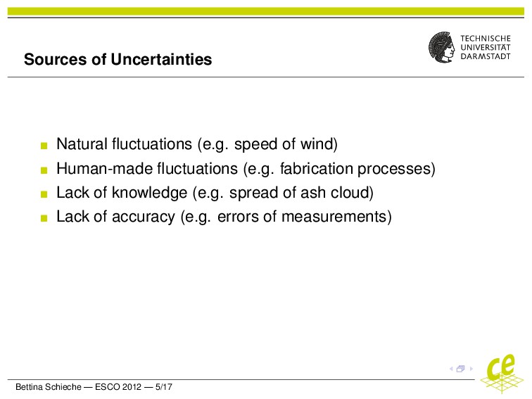
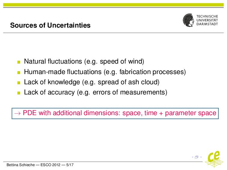
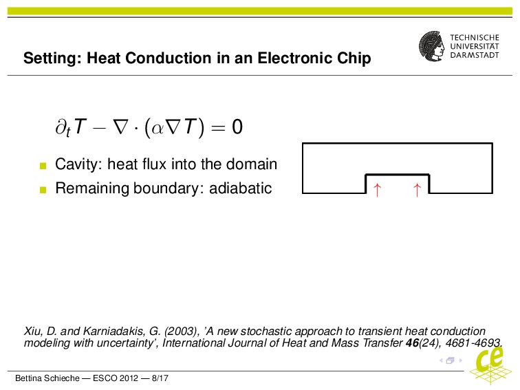
Numerical simulations become more reliable if random effects are taken into account. To this end, uncertain parameters can be expressed by random variables or random fields, which leads to partial differential equations (PDEs) with random parameters.
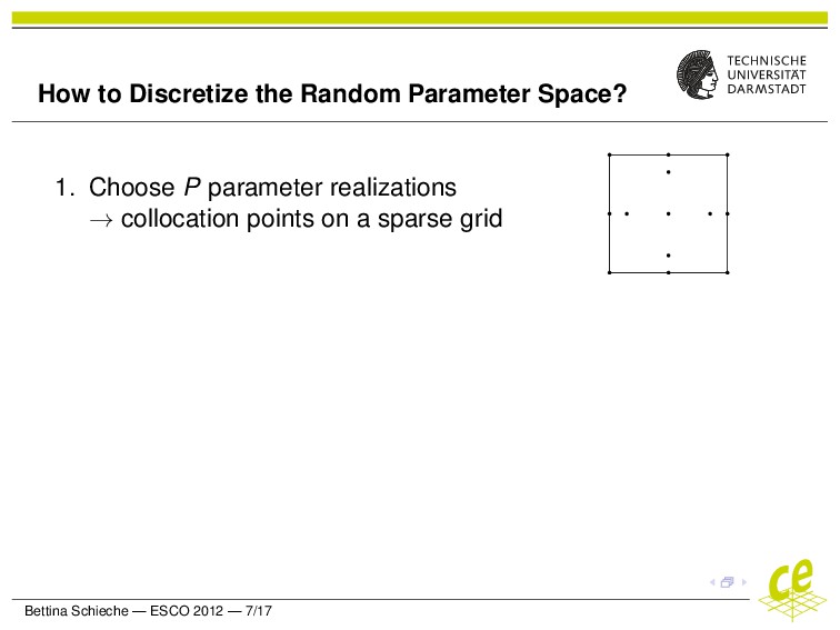
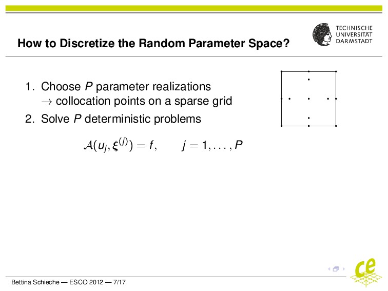
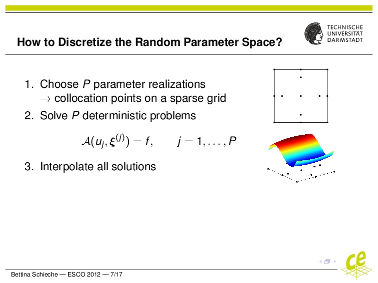
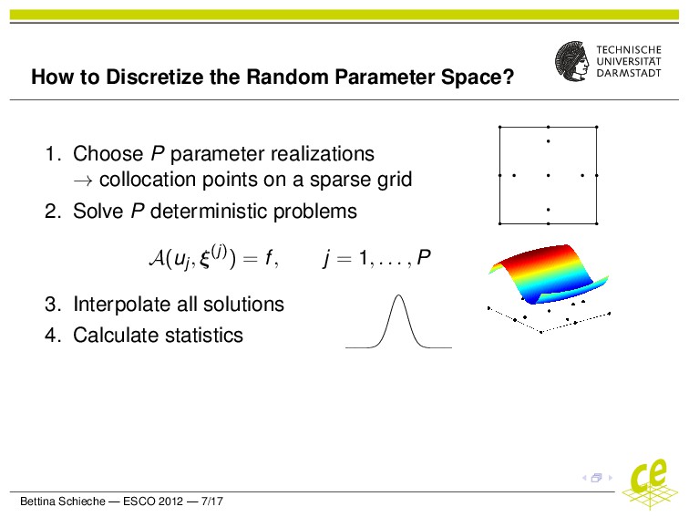
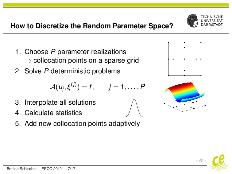
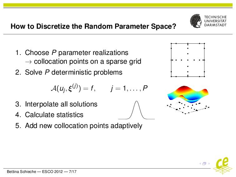
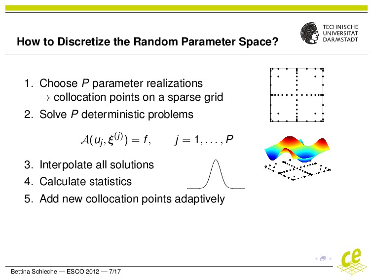
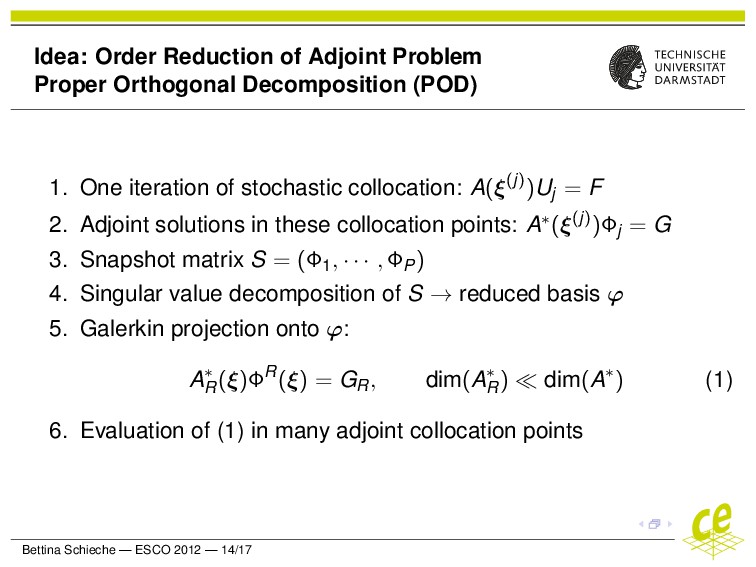
Common numerical methods to solve such problems are spectral methods of Galerkin type and stochastic collocation on sparse grids. We focus on the latter, because it decouples the random PDE into a set of deterministic equations.
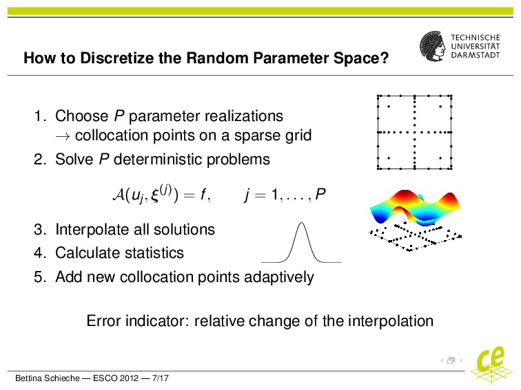
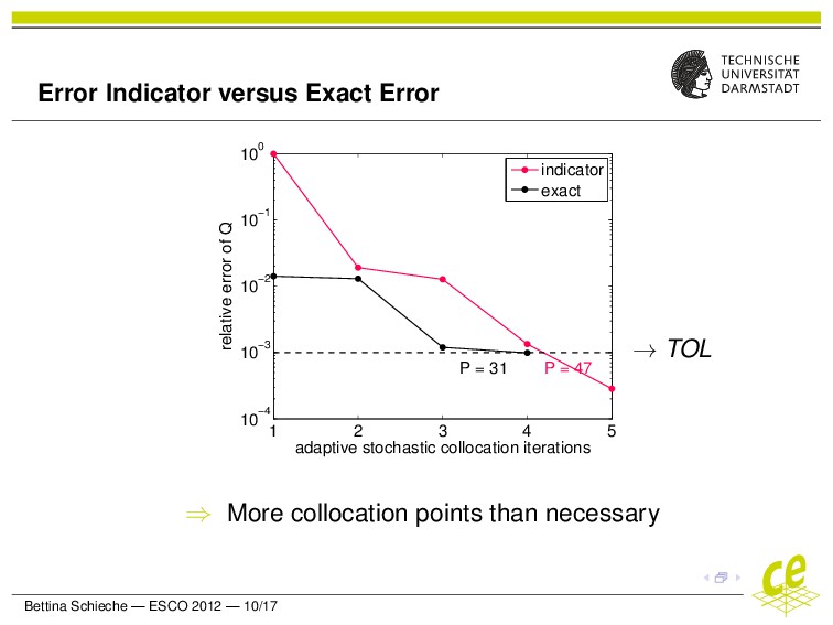
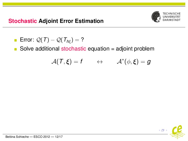
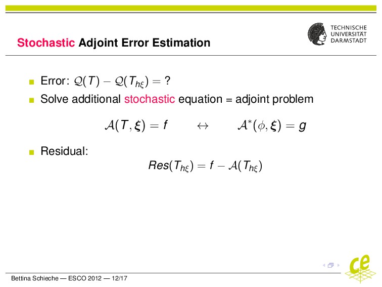
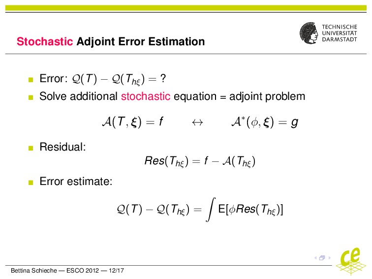
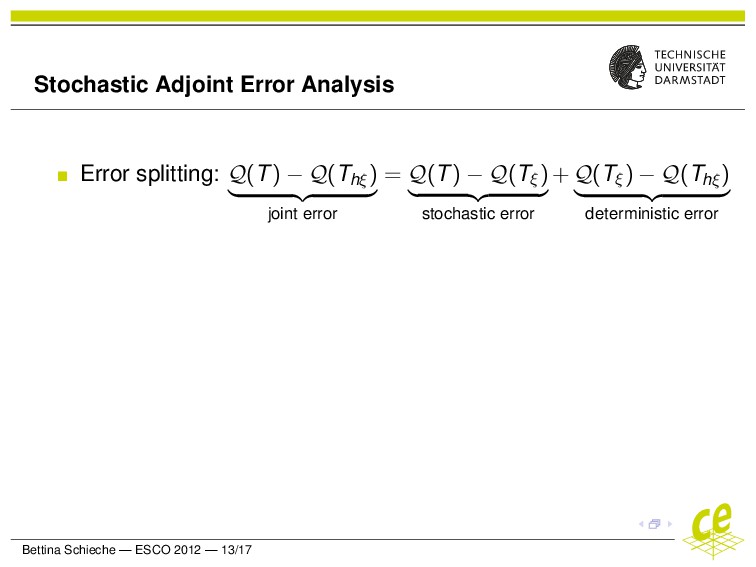
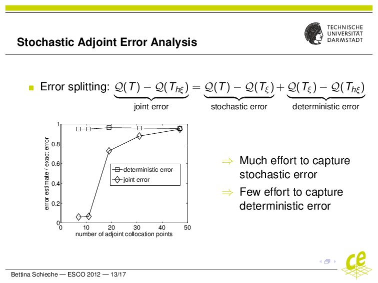
Our aim to analyze and improve adaptive stochastic collocation methods. A problem with adaptive strategies is to provide error estimates that capture both the deterministic and stochastic error, but are not too costly. A compromise between efficient error indicators and impractical error estimators is required.

Transcript

1. Analysis and Application of PDEs with Random Parameters Bettina Schieche Graduate School of Computational Engineering Numerical Analysis and Scientific Computing Technische Universit¨ at Darmstadt Numerical Analysis European Seminar on Computing Pilsen, Czech Republic, June 25 - 29, 2012 www.graduate-school-ce.de June 26, 2012
2. Outline Motivation for PDEs with Random Parameters Adaptive Stochastic Collocation Method Adjoint Error Estimation Bettina Schieche — ESCO 2012 — 2/17
3. Overview Motivation for PDEs with Random Parameters Adaptive Stochastic Collocation Method Adjoint Error Estimation Bettina Schieche — ESCO 2012 — 3/17
4. General Setting: Arbitrary PDE Describing parameters: Boundary and initial conditions Material properties Forcing terms / source terms Topology (geometry of the system) Bettina Schieche — ESCO 2012 — 4/17
5. Sources of Uncertainties Natural fluctuations (e.g. speed of wind) Human-made fluctuations (e.g. fabrication processes) Lack of knowledge (e.g. spread of ash cloud) Lack of accuracy (e.g. errors of measurements) Bettina Schieche — ESCO 2012 — 5/17
6. Sources of Uncertainties Natural fluctuations (e.g. speed of wind) Human-made fluctuations (e.g. fabrication processes) Lack of knowledge (e.g. spread of ash cloud) Lack of accuracy (e.g. errors of measurements) → PDE with additional dimensions: space, time + parameter space Bettina Schieche — ESCO 2012 — 5/17
7. Overview Motivation for PDEs with Random Parameters Adaptive Stochastic Collocation Method Adjoint Error Estimation Bettina Schieche — ESCO 2012 — 6/17
8. How to Discretize the Random Parameter Space? 1. Choose P parameter realizations → collocation points on a sparse grid Bettina Schieche — ESCO 2012 — 7/17
9. How to Discretize the Random Parameter Space? 1. Choose P parameter realizations → collocation points on a sparse grid 2. Solve P deterministic problems A(uj, ξ(j)) = f, j = 1, . . . , P Bettina Schieche — ESCO 2012 — 7/17
10. How to Discretize the Random Parameter Space? 1. Choose P parameter realizations → collocation points on a sparse grid 2. Solve P deterministic problems A(uj, ξ(j)) = f, j = 1, . . . , P 3. Interpolate all solutions Bettina Schieche — ESCO 2012 — 7/17
11. How to Discretize the Random Parameter Space? 1. Choose P parameter realizations → collocation points on a sparse grid 2. Solve P deterministic problems A(uj, ξ(j)) = f, j = 1, . . . , P 3. Interpolate all solutions 4. Calculate statistics Bettina Schieche — ESCO 2012 — 7/17
12. How to Discretize the Random Parameter Space? 1. Choose P parameter realizations → collocation points on a sparse grid 2. Solve P deterministic problems A(uj, ξ(j)) = f, j = 1, . . . , P 3. Interpolate all solutions 4. Calculate statistics 5. Add new collocation points adaptively Bettina Schieche — ESCO 2012 — 7/17
13. How to Discretize the Random Parameter Space? 1. Choose P parameter realizations → collocation points on a sparse grid 2. Solve P deterministic problems A(uj, ξ(j)) = f, j = 1, . . . , P 3. Interpolate all solutions 4. Calculate statistics 5. Add new collocation points adaptively Bettina Schieche — ESCO 2012 — 7/17
14. How to Discretize the Random Parameter Space? 1. Choose P parameter realizations → collocation points on a sparse grid 2. Solve P deterministic problems A(uj, ξ(j)) = f, j = 1, . . . , P 3. Interpolate all solutions 4. Calculate statistics 5. Add new collocation points adaptively Bettina Schieche — ESCO 2012 — 7/17
15. How to Discretize the Random Parameter Space? 1. Choose P parameter realizations → collocation points on a sparse grid 2. Solve P deterministic problems A(uj, ξ(j)) = f, j = 1, . . . , P 3. Interpolate all solutions 4. Calculate statistics 5. Add new collocation points adaptively Error indicator: relative change of the interpolation Bettina Schieche — ESCO 2012 — 7/17
16. Setting: Heat Conduction in an Electronic Chip ↑ ↑ ∂t T − ∇ · (α∇T) = 0 Cavity: heat flux into the domain Remaining boundary: adiabatic Xiu, D. and Karniadakis, G. (2003), ’A new stochastic approach to transient heat conduction modeling with uncertainty’, International Journal of Heat and Mass Transfer 46(24), 4681-4693. Bettina Schieche — ESCO 2012 — 8/17
17. Setting: Heat Conduction in an Electronic Chip ↑ ↑ ∂t T − ∇ · (α∇T) = 0 Cavity: heat flux into the domain Remaining boundary: adiabatic α random field: α(x, ξ1, ξ2, ξ3) = E[α] + σ 3 n=1 fn(x)ξn Xiu, D. and Karniadakis, G. (2003), ’A new stochastic approach to transient heat conduction modeling with uncertainty’, International Journal of Heat and Mass Transfer 46(24), 4681-4693. Bettina Schieche — ESCO 2012 — 8/17
18. Setting: Heat Conduction in an Electronic Chip ↑ ↑ ∂t T − ∇ · (α∇T) = 0 Cavity: heat flux into the domain Remaining boundary: adiabatic α random field: α(x, ξ1, ξ2, ξ3) = E[α] + σ 3 n=1 fn(x)ξn ξn independent, uniformly distributed Xiu, D. and Karniadakis, G. (2003), ’A new stochastic approach to transient heat conduction modeling with uncertainty’, International Journal of Heat and Mass Transfer 46(24), 4681-4693. Bettina Schieche — ESCO 2012 — 8/17
19. Setting: Heat Conduction in an Electronic Chip ↑ ↑ ∂t T − ∇ · (α∇T) = 0 Cavity: heat flux into the domain Remaining boundary: adiabatic α random field: α(x, ξ1, ξ2, ξ3) = E[α] + σ 3 n=1 fn(x)ξn ξn independent, uniformly distributed E[α] = 1, σ = 0.2 Xiu, D. and Karniadakis, G. (2003), ’A new stochastic approach to transient heat conduction modeling with uncertainty’, International Journal of Heat and Mass Transfer 46(24), 4681-4693. Bettina Schieche — ESCO 2012 — 8/17
20. Adaptive Stochastic Collocation: First Results Stochastic collocation approximation → Thξ Results at time t = 1: Expected Value Standard Deviation Bettina Schieche — ESCO 2012 — 9/17
21. Adaptive Stochastic Collocation: First Results Stochastic collocation approximation → Thξ Results at time t = 1: Expected Value Standard Deviation (0, 0) Quantity of interest: Q(T) = Var[ 1 0 T|x=(0,0) dt] Aim: Q(T) − Q(Thξ ) ! < TOL = 10−3 Bettina Schieche — ESCO 2012 — 9/17
22. Error Indicator versus Exact Error 1 2 3 4 5 10−4 10−3 10−2 10−1 100 P = 47 P = 31 adaptive stochastic collocation iterations relative error of Q indicator exact ⇒ More collocation points than necessary → TOL Bettina Schieche — ESCO 2012 — 10/17
23. Overview Motivation for PDEs with Random Parameters Adaptive Stochastic Collocation Method Adjoint Error Estimation Bettina Schieche — ESCO 2012 — 11/17
24. Stochastic Adjoint Error Estimation Error: Q(T) − Q(Thξ ) = ? Bettina Schieche — ESCO 2012 — 12/17
25. Stochastic Adjoint Error Estimation Error: Q(T) − Q(Thξ ) = ? Solve additional stochastic equation = adjoint problem A(T, ξ) = f ↔ A∗(φ, ξ) = g Bettina Schieche — ESCO 2012 — 12/17
26. Stochastic Adjoint Error Estimation Error: Q(T) − Q(Thξ ) = ? Solve additional stochastic equation = adjoint problem A(T, ξ) = f ↔ A∗(φ, ξ) = g Residual: Res(Thξ ) = f − A(Thξ ) Bettina Schieche — ESCO 2012 — 12/17
27. Stochastic Adjoint Error Estimation Error: Q(T) − Q(Thξ ) = ? Solve additional stochastic equation = adjoint problem A(T, ξ) = f ↔ A∗(φ, ξ) = g Residual: Res(Thξ ) = f − A(Thξ ) Error estimate: Q(T) − Q(Thξ ) = E[φRes(Thξ )] Bettina Schieche — ESCO 2012 — 12/17
28. Stochastic Adjoint Error Analysis Error splitting: Q(T) − Q(Thξ ) joint error = Q(T) − Q(Tξ) stochastic error + Q(Tξ) − Q(Thξ ) deterministic error Bettina Schieche — ESCO 2012 — 13/17
29. Stochastic Adjoint Error Analysis Error splitting: Q(T) − Q(Thξ ) joint error = Q(T) − Q(Tξ) stochastic error + Q(Tξ) − Q(Thξ ) deterministic error 0 10 20 30 40 50 0 0.2 0.4 0.6 0.8 1 number of adjoint collocation points error estimate / exact error deterministic error joint error ⇒ Much effort to capture stochastic error ⇒ Few effort to capture deterministic error Bettina Schieche — ESCO 2012 — 13/17
30. Idea: Order Reduction of Adjoint Problem Proper Orthogonal Decomposition (POD) 1. One iteration of stochastic collocation: A(ξ(j))Uj = F 2. Adjoint solutions in these collocation points: A∗(ξ(j))Φj = G 3. Snapshot matrix S = (Φ1, · · · , ΦP) 4. Singular value decomposition of S → reduced basis ϕ 5. Galerkin projection onto ϕ: A∗ R (ξ)ΦR(ξ) = GR, dim(A∗ R ) dim(A∗) (1) 6. Evaluation of (1) in many adjoint collocation points Bettina Schieche — ESCO 2012 — 14/17
31. Error Indicator versus Adjoint Error Estimator 1 2 3 4 5 10−4 10−3 10−2 10−1 100 P = 47 P = 31 adaptive stochastic collocation iterations relative error of Q indicator exact reduced adjoint ⇒ Reduced adjoints very close to exact error → TOL Bettina Schieche — ESCO 2012 — 15/17
32. POD Modes of the Stochastic Adjoint Solution 1 2 3 4 5 6 7 8 9 Bettina Schieche — ESCO 2012 — 16/17
33. Conclusion & Outlook Stochastic collocation results in a set of deterministic equations. Full adjoint stochastic collocation is usually not practicable. Reduced order models can reduce computational costs. Bettina Schieche — ESCO 2012 — 17/17
34. Conclusion & Outlook Stochastic collocation results in a set of deterministic equations. Full adjoint stochastic collocation is usually not practicable. Reduced order models can reduce computational costs. ⇒ Order reduction of the primal problem ⇒ Local reconstruction of adjoint solutions Bettina Schieche — ESCO 2012 — 17/17
35. Conclusion & Outlook Stochastic collocation results in a set of deterministic equations. Full adjoint stochastic collocation is usually not practicable. Reduced order models can reduce computational costs. ⇒ Order reduction of the primal problem ⇒ Local reconstruction of adjoint solutions The work is supported by the “Excellence Initiative“ of the German Federal and State Governments and the Graduate School of Computational Engineering at TU Darmstadt. Bettina Schieche — ESCO 2012 — 17/17