Analysis and Application of PDEs with Random Parameters

An overview of PDEs with random input data with a focus on adaptive stochastic collocation

Transcript

1. Analysis and Application of PDEs with Random Parameters Bettina Schieche, Jens Lang Technische Universit¨ at Darmstadt Fachbereich Mathematik Arbeitsgruppe Numerik und Wissenschaftliches Rechnen 20. Treffen des Rhein-Main Arbeitskreises Frankfurt, den 18. Januar 2013 www.mathematik.tu-darmstadt.de
2. Applications for Random Parameters diffusion coefficients chemical reactions: reaction coefficients porous media: permeability rough surfaces: boundary deviations fluid mechanics: boundary conditions Bettina Schieche | 18.01.13 | Motivation | 2/28
3. Contents Problem Formulation Exact Calculation of Moments Adaptive Stochastic Collocation Bettina Schieche | 18.01.13 | Contents | 3/28
4. Overview Problem Formulation Exact Calculation of Moments Adaptive Stochastic Collocation Bettina Schieche | 18.01.13 | Problem Formulation | 4/28
5. Deterministic Problem 1. A(u, α(x)) = f ⇒ u(x) – parameter α – solution space e.g. Banach space X Bettina Schieche | 18.01.13 | Problem Formulation | 5/28
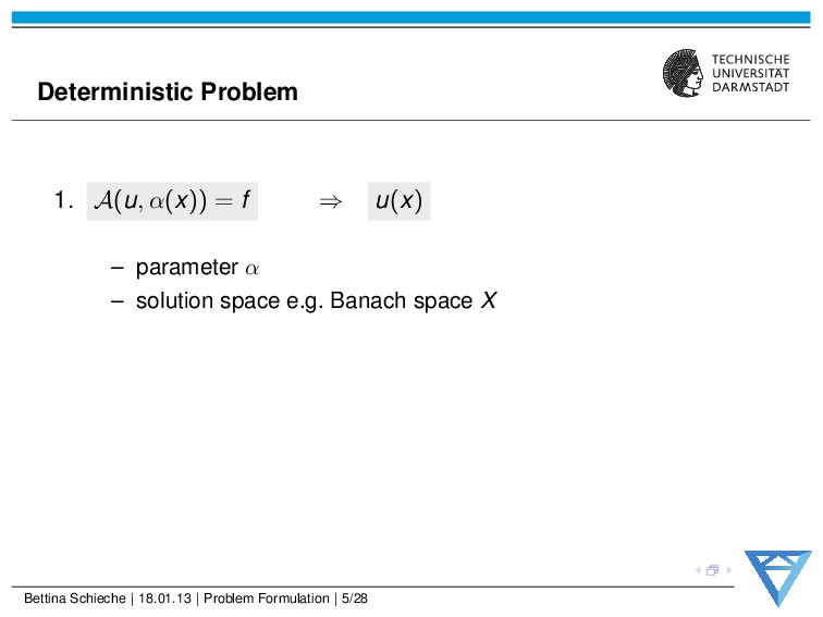
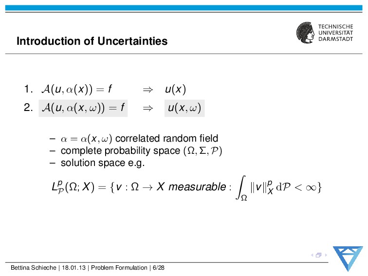
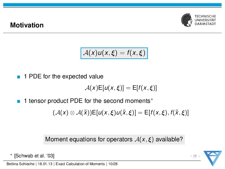
6. Introduction of Uncertainties 1. A(u, α(x)) = f ⇒ u(x) 2. A(u, α(x, ω)) = f ⇒ u(x, ω) – α = α(x, ω) correlated random field – complete probability space (Ω, Σ, P) – solution space e.g. Lp P (Ω; X) = {v : Ω → X measurable : Ω v p X dP < ∞} Bettina Schieche | 18.01.13 | Problem Formulation | 6/28
7. “Finite-Noise-Assumption” 1. A(u, α(x)) = f ⇒ u(x) 2. A(u, α(x, ω)) = f ⇒ u(x, ω) 3. A(u, α(x, ξ)) = f ⇒ u(x, ξ) – α(x, ω) = ∞ n=1 fn(x)ξn(ω) (Karhunen-Lo` eve expansion, . . . ) – α(x, ξ) = M n=1 fn(x)ξn , ξ = (ξ1, . . . , ξM ) – stochastic independence Bettina Schieche | 18.01.13 | Problem Formulation | 7/28
8. Transformation onto the Image Measure 1. A(u, α(x)) = f ⇒ u(x) 2. A(u, α(x, ω)) = f ⇒ u(x, ω) 3. A(u, α(x, ξ)) = f ⇒ u(x, ξ) 4. A(u, α(x, y)) = f ⇒ u(x, y) – density function ρ(y) – parameter space Γ := ξ1(Ω) × · · · × ξM (Ω) ⊆ RM y1 y2 Bettina Schieche | 18.01.13 | Problem Formulation | 8/28
9. Overview Problem Formulation Exact Calculation of Moments Adaptive Stochastic Collocation Bettina Schieche | 18.01.13 | Exact Calculation of Moments | 9/28
10. Motivation A(x)u(x, ξ) = f(x, ξ) 1 PDE for the expected value A(x)E[u(x, ξ)] = E[f(x, ξ)] 1 tensor product PDE for the second moments∗ (A(x) ⊗ A(˜ x))E[u(x, ξ)u(˜ x, ξ)] = E[f(x, ξ), f(˜ x, ξ)] ∗ [Schwab et al. ’03] Bettina Schieche | 18.01.13 | Exact Calculation of Moments | 10/28
11. Motivation A(x)u(x, ξ) = f(x, ξ) 1 PDE for the expected value A(x)E[u(x, ξ)] = E[f(x, ξ)] 1 tensor product PDE for the second moments∗ (A(x) ⊗ A(˜ x))E[u(x, ξ)u(˜ x, ξ)] = E[f(x, ξ), f(˜ x, ξ)] Moment equations for operators A(x, ξ) available? ∗ [Schwab et al. ’03] Bettina Schieche | 18.01.13 | Exact Calculation of Moments | 10/28
12. Weighted Operator ∂t v = ξAv v(0) = v0 ⇒ ∂t E[v] =A E[ξv] Bettina Schieche | 18.01.13 | Exact Calculation of Moments | 11/28
13. Weighted Operator ∂t v = ξAv v(0) = v0 ⇒ ∂t E[v] =A E[ξv] but: E[v] = b a v(t, y)ρ(y) dy Bettina Schieche | 18.01.13 | Exact Calculation of Moments | 11/28
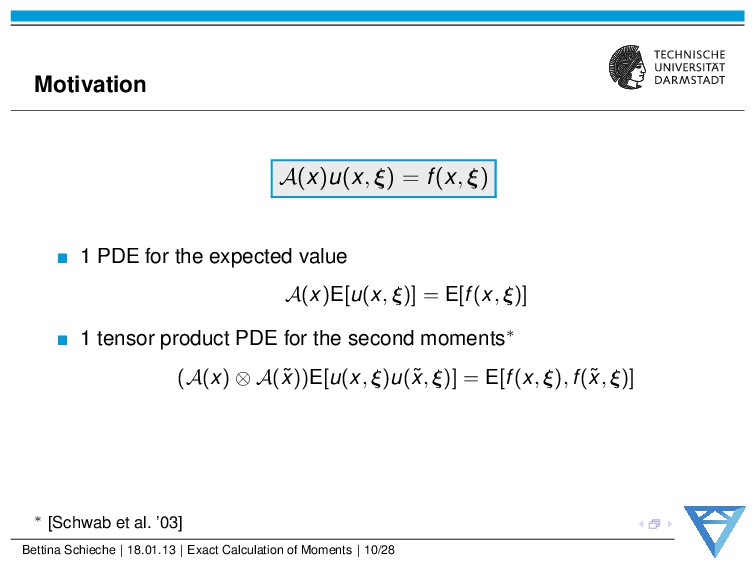
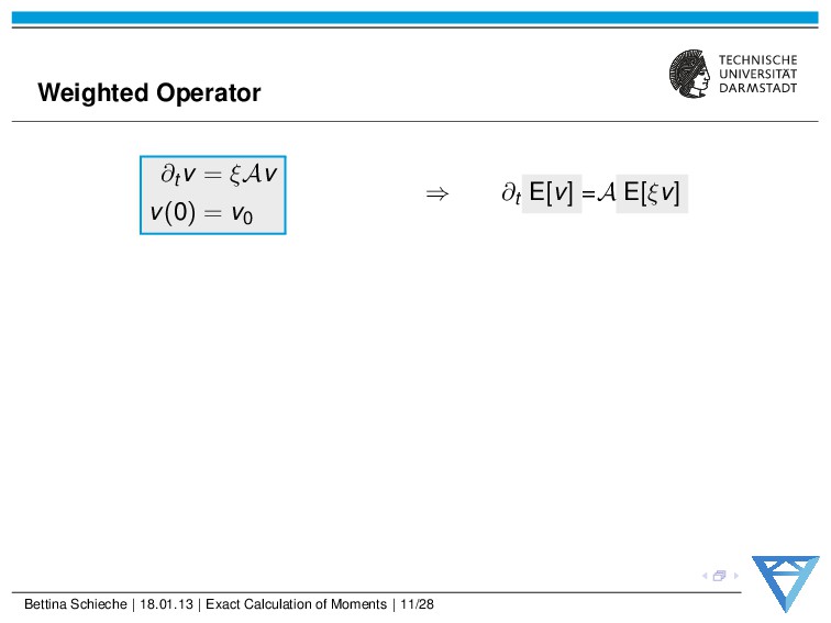
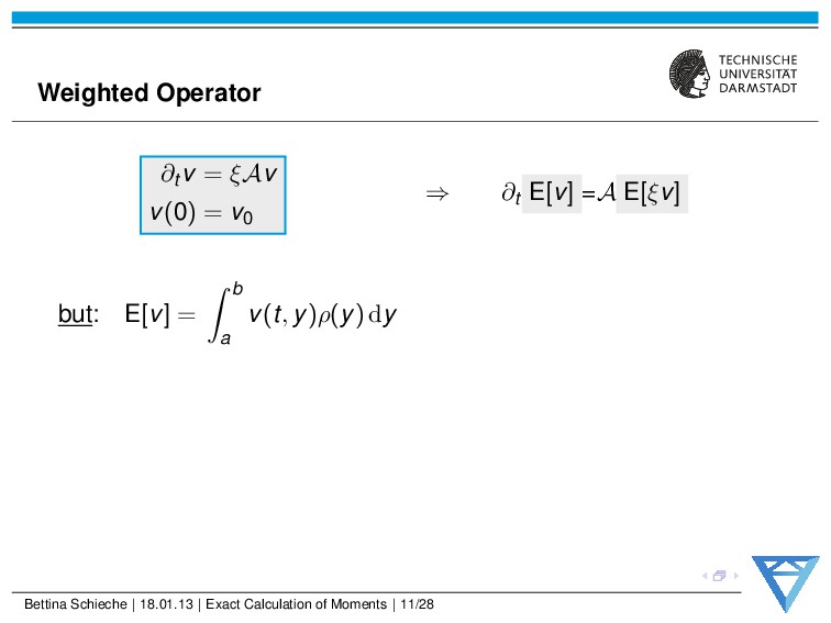
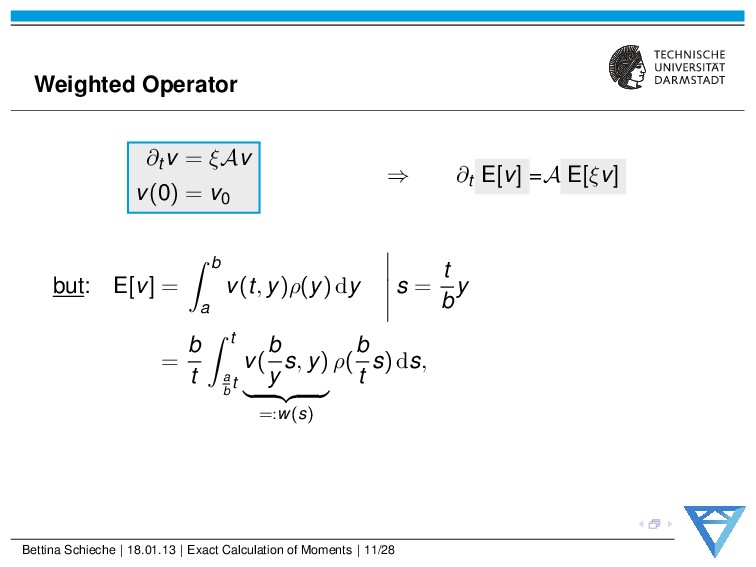
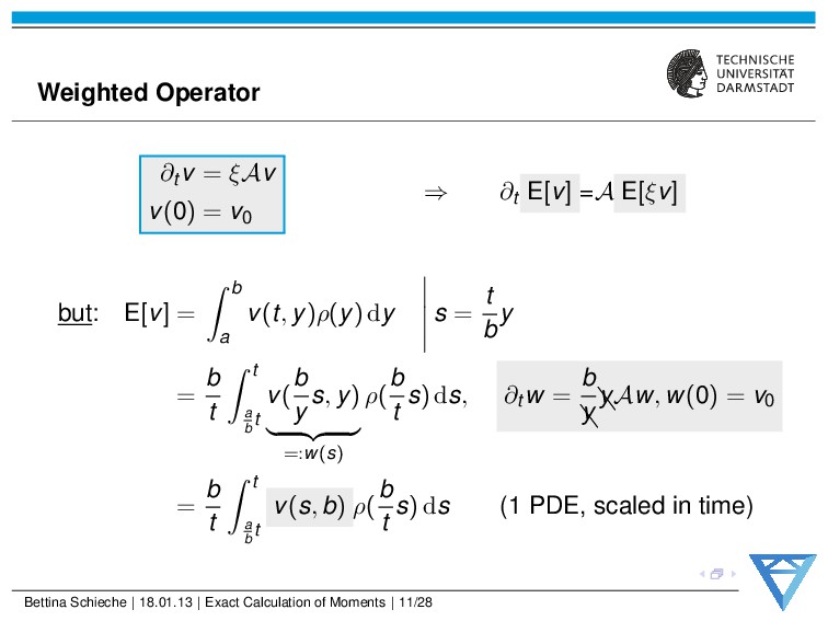
14. Weighted Operator ∂t v = ξAv v(0) = v0 ⇒ ∂t E[v] =A E[ξv] but: E[v] = b a v(t, y)ρ(y) dy s = t b y = b t t a b t v( b y s, y) =:w(s) ρ( b t s) ds, Bettina Schieche | 18.01.13 | Exact Calculation of Moments | 11/28
15. Weighted Operator ∂t v = ξAv v(0) = v0 ⇒ ∂t E[v] =A E[ξv] but: E[v] = b a v(t, y)ρ(y) dy s = t b y = b t t a b t v( b y s, y) =:w(s) ρ( b t s) ds, ∂t w = b S S y S S yAw, w(0) = v0 = b t t a b t v(s, b) ρ( b t s) ds (1 PDE, scaled in time) Bettina Schieche | 18.01.13 | Exact Calculation of Moments | 11/28
16. Sum of 2 Operators ∂t v = (A0 + ξA1) v, ξ ∼ U[−a, a] v(0) = v0 Bettina Schieche | 18.01.13 | Exact Calculation of Moments | 12/28
17. Sum of 2 Operators ∂t v = (A0 + ξA1) v, ξ ∼ U[−a, a] v(0) = v0 E[v] = 1 2a a −a v(t, y) dy Bettina Schieche | 18.01.13 | Exact Calculation of Moments | 12/28
18. Sum of 2 Operators ∂t v = (A0 + ξA1) v, ξ ∼ U[−a, a] v(0) = v0 E[v] = 1 2a a −a v(t, y) dy = 1 2a 0 −a v(t, y) dy + a 0 v(t, y) dy Bettina Schieche | 18.01.13 | Exact Calculation of Moments | 12/28
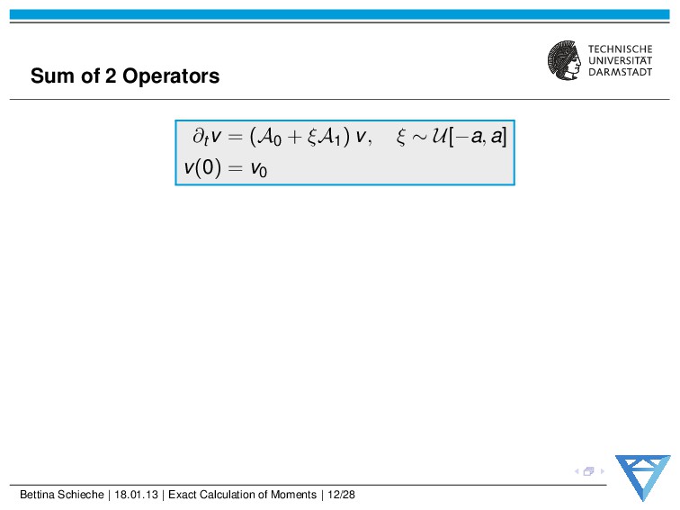
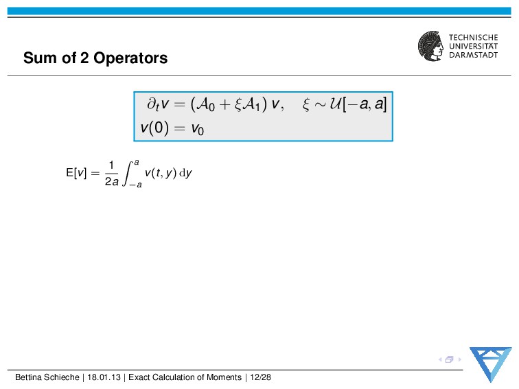
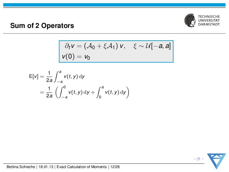
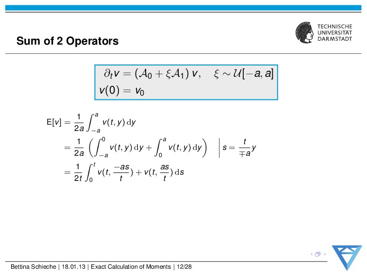
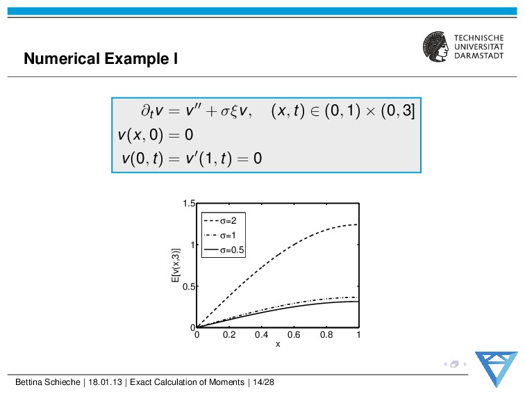
19. Sum of 2 Operators ∂t v = (A0 + ξA1) v, ξ ∼ U[−a, a] v(0) = v0 E[v] = 1 2a a −a v(t, y) dy = 1 2a 0 −a v(t, y) dy + a 0 v(t, y) dy s = t ∓a y = 1 2t t 0 v(t, −as t ) + v(t, as t ) ds Bettina Schieche | 18.01.13 | Exact Calculation of Moments | 12/28
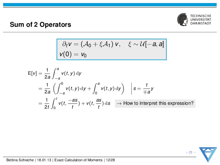
20. Sum of 2 Operators ∂t v = (A0 + ξA1) v, ξ ∼ U[−a, a] v(0) = v0 E[v] = 1 2a a −a v(t, y) dy = 1 2a 0 −a v(t, y) dy + a 0 v(t, y) dy s = t ∓a y = 1 2t t 0 v(t, −as t ) + v(t, as t ) ds → How to interpret this expression? Bettina Schieche | 18.01.13 | Exact Calculation of Moments | 12/28
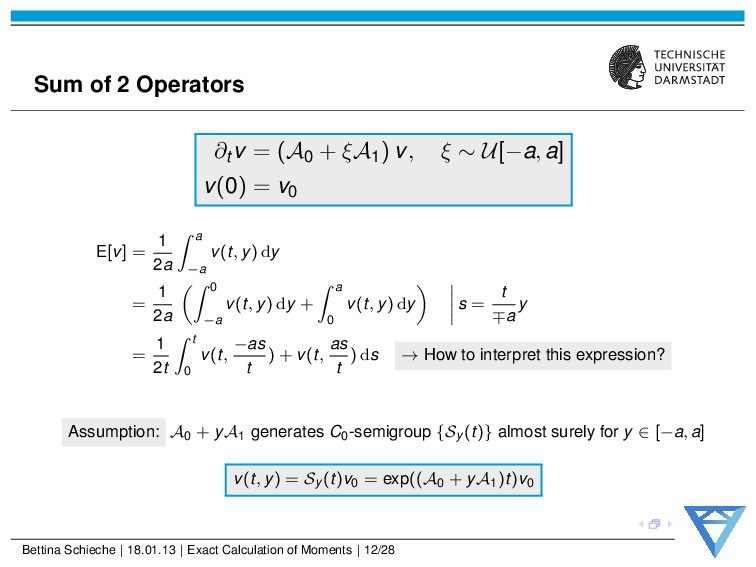
21. Sum of 2 Operators ∂t v = (A0 + ξA1) v, ξ ∼ U[−a, a] v(0) = v0 E[v] = 1 2a a −a v(t, y) dy = 1 2a 0 −a v(t, y) dy + a 0 v(t, y) dy s = t ∓a y = 1 2t t 0 v(t, −as t ) + v(t, as t ) ds → How to interpret this expression? Assumption: A0 + yA1 generates C0-semigroup {Sy (t)} almost surely for y ∈ [−a, a] v(t, y) = Sy (t)v0 = exp((A0 + yA1)t)v0 Bettina Schieche | 18.01.13 | Exact Calculation of Moments | 12/28
22. Sum of 2 Operators: Main Result Theorem: A0, A1 commutative ⇒ E[v] = 1 2t u, ∂t u = A0u + v(t, −a) + v(t, a) u(0) = 0 Bettina Schieche | 18.01.13 | Exact Calculation of Moments | 13/28
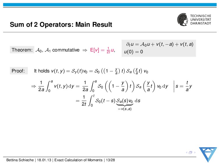
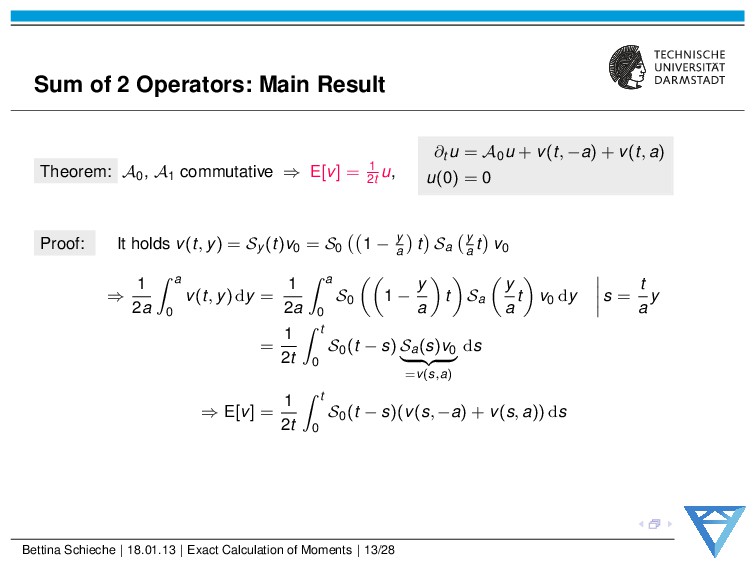
23. Sum of 2 Operators: Main Result Theorem: A0, A1 commutative ⇒ E[v] = 1 2t u, ∂t u = A0u + v(t, −a) + v(t, a) u(0) = 0 Proof: It holds v(t, y) = Sy (t)v0 = S0 1 − y a t Sa y a t v0 ⇒ 1 2a a 0 v(t, y) dy = 1 2a a 0 S0 1 − y a t Sa y a t v0 dy s = t a y = 1 2t t 0 S0(t − s) Sa(s)v0 =v(s,a) ds Bettina Schieche | 18.01.13 | Exact Calculation of Moments | 13/28
24. Sum of 2 Operators: Main Result Theorem: A0, A1 commutative ⇒ E[v] = 1 2t u, ∂t u = A0u + v(t, −a) + v(t, a) u(0) = 0 Proof: It holds v(t, y) = Sy (t)v0 = S0 1 − y a t Sa y a t v0 ⇒ 1 2a a 0 v(t, y) dy = 1 2a a 0 S0 1 − y a t Sa y a t v0 dy s = t a y = 1 2t t 0 S0(t − s) Sa(s)v0 =v(s,a) ds ⇒ E[v] = 1 2t t 0 S0(t − s)(v(s, −a) + v(s, a)) ds Bettina Schieche | 18.01.13 | Exact Calculation of Moments | 13/28
25. Sum of 2 Operators: Main Result Theorem: A0, A1 commutative ⇒ E[v] = 1 2t u, ∂t u = A0u + v(t, −a) + v(t, a) u(0) = 0 Proof: It holds v(t, y) = Sy (t)v0 = S0 1 − y a t Sa y a t v0 ⇒ 1 2a a 0 v(t, y) dy = 1 2a a 0 S0 1 − y a t Sa y a t v0 dy s = t a y = 1 2t t 0 S0(t − s) Sa(s)v0 =v(s,a) ds ⇒ E[v] = 1 2t t 0 S0(t − s)(v(s, −a) + v(s, a)) ds Variation of constants completes the proof. (2+1 PDEs to be solved) Bettina Schieche | 18.01.13 | Exact Calculation of Moments | 13/28
26. Numerical Example I ∂t v = v + σξv, (x, t) ∈ (0, 1) × (0, 3] v(x, 0) = 0 v(0, t) = v (1, t) = 0 0 0.2 0.4 0.6 0.8 1 0 0.5 1 1.5 x E[v(x,3)] σ=2 σ=1 σ=0.5 Bettina Schieche | 18.01.13 | Exact Calculation of Moments | 14/28
27. Chances and Limits of the Approach Chances: A(ξ) = A0 + M n=1 ξnAn , commuting operators → 3M PDEs to be solved iteratively inhomogeneous terms of the type f(t)g(x) Limits: higher moments arbitrary inhomogeneous terms arbitrary distributions (non-commuting operators . . . ) Bettina Schieche | 18.01.13 | Exact Calculation of Moments | 15/28
28. . . . Non-Commuting Operators: Numerical Example II ∂t v = (1 + f(x)σξ)v , (x, t) ∈ (0, 1) × (0, 0.1] v(x, 0) = 4x(1 − x) v(0, t) = v(1, t) = 0 10−2 10−1 100 10−6 10−5 10−4 10−3 10−2 σ max. relative error E[v] O(σ2) Bettina Schieche | 18.01.13 | Exact Calculation of Moments | 16/28
29. Overview Problem Formulation Exact Calculation of Moments Adaptive Stochastic Collocation Bettina Schieche | 18.01.13 | Adaptive Stochastic Collocation | 17/28
30. Stochastic Collocation: General Procedure 1. P realizations: {y(j)}P j=1 → collocation points Bettina Schieche | 18.01.13 | Adaptive Stochastic Collocation | 18/28
31. Stochastic Collocation: General Procedure 1. P realizations: {y(j)}P j=1 → collocation points 2. P deterministic problems A(uj, α(x, y(j)) = f, uj := u(x, y(j)), j = 1, . . . , P Bettina Schieche | 18.01.13 | Adaptive Stochastic Collocation | 18/28
32. Stochastic Collocation: General Procedure 1. P realizations: {y(j)}P j=1 → collocation points 2. P deterministic problems A(uj, α(x, y(j)) = f, uj := u(x, y(j)), j = 1, . . . , P 3. interpolation of all solutions Bettina Schieche | 18.01.13 | Adaptive Stochastic Collocation | 18/28
33. Stochastic Collocation: General Procedure 1. P realizations: {y(j)}P j=1 → collocation points 2. P deterministic problems A(uj, α(x, y(j)) = f, uj := u(x, y(j)), j = 1, . . . , P 3. interpolation of all solutions 4. calculation of statistical quantities: quadrature Bettina Schieche | 18.01.13 | Adaptive Stochastic Collocation | 18/28
34. Stochastic Collocation: General Procedure 1. P realizations: {y(j)}P j=1 → collocation points 2. P deterministic problems A(uj, α(x, y(j)) = f, uj := u(x, y(j)), j = 1, . . . , P 3. interpolation of all solutions 4. calculation of statistical quantities: quadrature 5. adaptive addition of new collocation points Bettina Schieche | 18.01.13 | Adaptive Stochastic Collocation | 18/28
35. Stochastic Collocation: General Procedure 1. P realizations: {y(j)}P j=1 → collocation points 2. P deterministic problems A(uj, α(x, y(j)) = f, uj := u(x, y(j)), j = 1, . . . , P 3. interpolation of all solutions 4. calculation of statistical quantities: quadrature 5. adaptive addition of new collocation points Bettina Schieche | 18.01.13 | Adaptive Stochastic Collocation | 18/28
36. Full and Sparse Grids Bettina Schieche | 18.01.13 | Adaptive Stochastic Collocation | 19/28
37. Full and Sparse Grids full, isotropic Bettina Schieche | 18.01.13 | Adaptive Stochastic Collocation | 19/28
38. Full and Sparse Grids full, isotropic Bettina Schieche | 18.01.13 | Adaptive Stochastic Collocation | 19/28
39. Full and Sparse Grids full, isotropic Bettina Schieche | 18.01.13 | Adaptive Stochastic Collocation | 19/28
40. Full and Sparse Grids full, isotropic Bettina Schieche | 18.01.13 | Adaptive Stochastic Collocation | 19/28
41. Full and Sparse Grids sparse, isotropic Bettina Schieche | 18.01.13 | Adaptive Stochastic Collocation | 19/28
42. Full and Sparse Grids sparse, isotropic Bettina Schieche | 18.01.13 | Adaptive Stochastic Collocation | 19/28
43. Full and Sparse Grids sparse, isotropic Bettina Schieche | 18.01.13 | Adaptive Stochastic Collocation | 19/28
44. Full and Sparse Grids full, anisotropic Bettina Schieche | 18.01.13 | Adaptive Stochastic Collocation | 19/28
45. Full and Sparse Grids sparse, anisotropic Bettina Schieche | 18.01.13 | Adaptive Stochastic Collocation | 19/28
46. Algorithmic Details suitable collocation points: → Clenshaw-Curtis, Gauss-Patterson parallel solutions of PDEs in each iteration: → arbitrary solver (black box) global interpolation (Lagrange) dimension adaptive refinement∗ with respect to a quantity of interest → error indicator: relative change ∗[Gerstner & Griebel ’03] Bettina Schieche | 18.01.13 | Adaptive Stochastic Collocation | 20/28
47. Numerical Example: Boussinesq Equation ∂u ∂t + (u · ∇)u − 2 Re div (u) + ∇p = − 1 Fr T g div u = 0 ∂T ∂t + (u · ∇)T − 1 Pe ∆T = 0 velocity u pressure p temperature T Re = 10, Pe = 20/3, Fr = 1/150∗ normalized gravitation vector g ↓ T = 1 (0,0) (10,0) T = 0 (0,1) ∗[Evans, Paolucci ’90] Bettina Schieche | 18.01.13 | Adaptive Stochastic Collocation | 21/28
48. Numerical Example: Boussinesq Equation ∂u ∂t + (u · ∇)u − 2 Re div (u) + ∇p = − 1 Fr T g div u = 0 ∂T ∂t + (u · ∇)T − 1 Pe ∆T = 0 velocity u pressure p temperature T Re = 10, Pe = 20/3, Fr = 1/150∗ normalized gravitation vector g ↓ T = 1 (0,0) (10,0) T = 0 (0,1) ∗[Evans, Paolucci ’90] Bettina Schieche | 18.01.13 | Adaptive Stochastic Collocation | 21/28
49. Numerical Example: Boussinesq Equation ∂u ∂t + (u · ∇)u − 2 Re div (u) + ∇p = − 1 Fr T g div u = 0 ∂T ∂t + (u · ∇)T − 1 Pe ∆T = 0 velocity u pressure p temperature T Re = 10, Pe = 20/3, Fr = 1/150∗ normalized gravitation vector g ↓ T = 1 (0,0) (10,0) T = 0 (0,1) ∗[Evans, Paolucci ’90] Bettina Schieche | 18.01.13 | Adaptive Stochastic Collocation | 21/28
50. Numerical Example: Boussinesq Equation ∂u ∂t + (u · ∇)u − 2 Re div (u) + ∇p = − 1 Fr T g div u = 0 ∂T ∂t + (u · ∇)T − 1 Pe ∆T = 0 velocity u pressure p temperature T Re = 10, Pe = 20/3, Fr = 1/150∗ normalized gravitation vector g ↓ T = 1 (0,0) (10,0) T = 0 (0,1) ∗[Evans, Paolucci ’90] Bettina Schieche | 18.01.13 | Adaptive Stochastic Collocation | 21/28
51. Numerical Example: Boussinesq Equation ∂u ∂t + (u · ∇)u − 2 Re div (u) + ∇p = − 1 Fr T g div u = 0 ∂T ∂t + (u · ∇)T − 1 Pe ∆T = 0 velocity u pressure p temperature T Re = 10, Pe = 20/3, Fr = 1/150∗ normalized gravitation vector g ↓ T = 1 (0,0) (10,0) T = 0 (0,1) ∗[Evans, Paolucci ’90] Bettina Schieche | 18.01.13 | Adaptive Stochastic Collocation | 21/28
52. Numerical Example: Boussinesq Equation ∂u ∂t + (u · ∇)u − 2 Re div (u) + ∇p = − 1 Fr T g div u = 0 ∂T ∂t + (u · ∇)T − 1 Pe ∆T = 0 velocity u pressure p temperature T Re = 10, Pe = 20/3, Fr = 1/150∗ normalized gravitation vector g ↓ T = 1 (0,0) (10,0) T = 0 (0,1) ∗[Evans, Paolucci ’90] Bettina Schieche | 18.01.13 | Adaptive Stochastic Collocation | 21/28
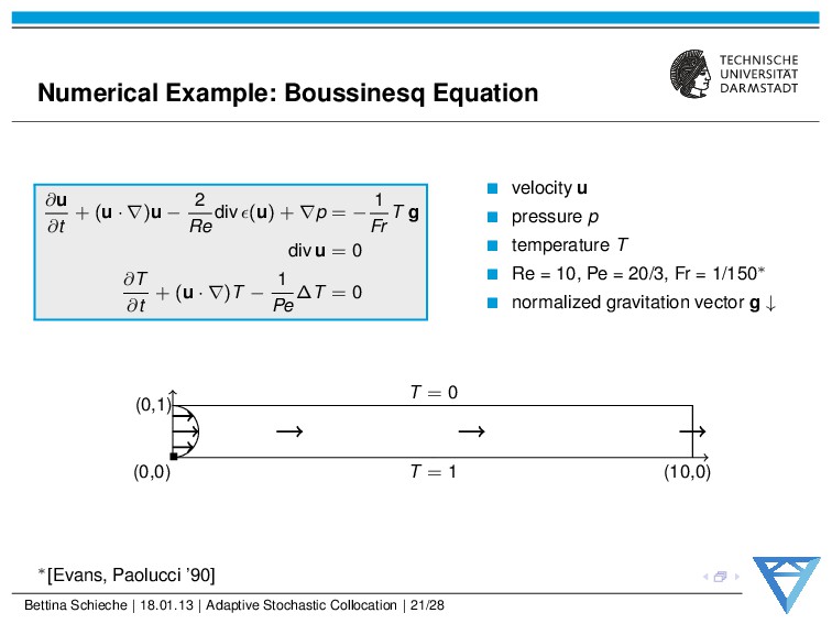
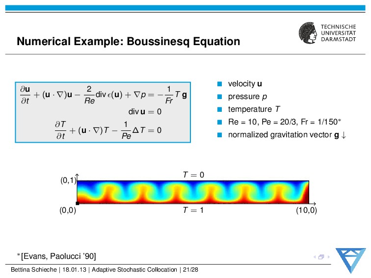
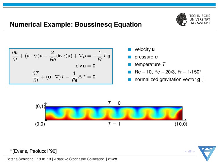
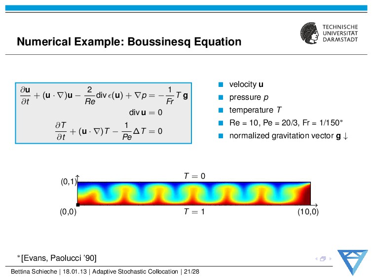
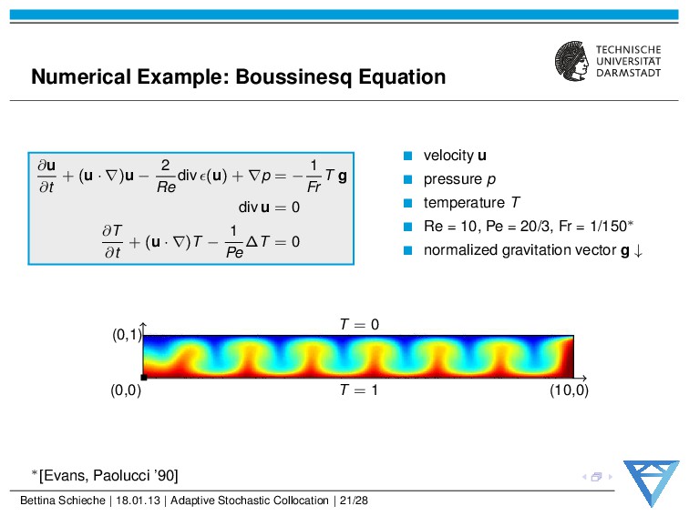
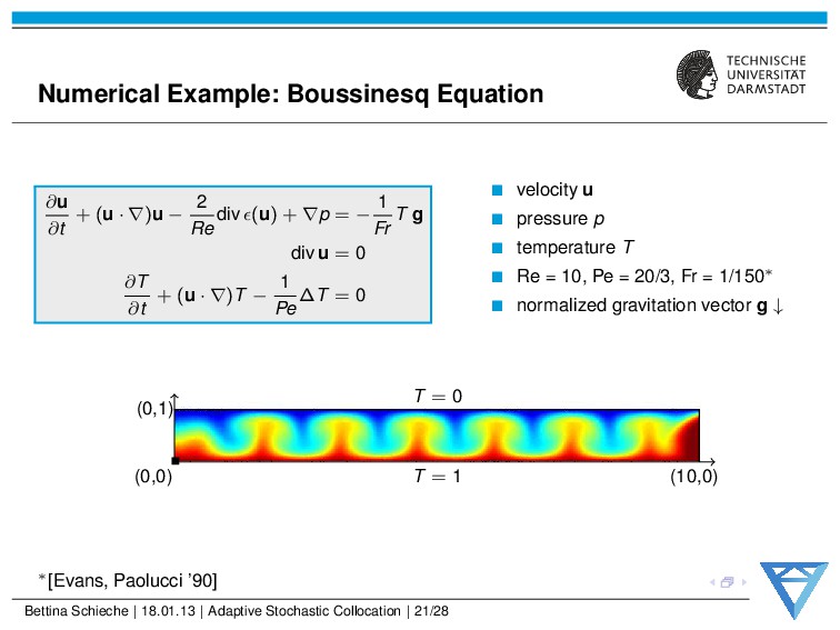
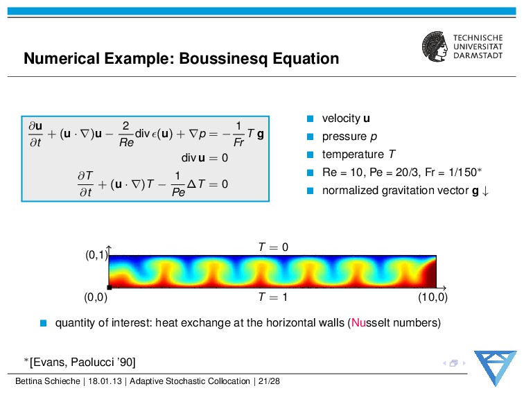
53. Numerical Example: Boussinesq Equation ∂u ∂t + (u · ∇)u − 2 Re div (u) + ∇p = − 1 Fr T g div u = 0 ∂T ∂t + (u · ∇)T − 1 Pe ∆T = 0 velocity u pressure p temperature T Re = 10, Pe = 20/3, Fr = 1/150∗ normalized gravitation vector g ↓ T = 1 (0,0) (10,0) T = 0 (0,1) quantity of interest: heat exchange at the horizontal walls (Nusselt numbers) ∗[Evans, Paolucci ’90] Bettina Schieche | 18.01.13 | Adaptive Stochastic Collocation | 21/28
54. Uncertain Boundary Condition T = 1 + σ M n=1 fn(x1)ξn (0,0) (10,0) T = 0 (0,1) ξn uniformly distributed correlation length L = 5, 10, 20 ⇒ M = 9, 5, 3 standard deviation σ = 0.125, 0.25, 0.5 Bettina Schieche | 18.01.13 | Adaptive Stochastic Collocation | 22/28
55. Uncertainty Quantification with respect to σ 0.125 0.25 0.5 10−3 10−2 10−1 100 101 standard deviation σ |E[Nu]−Nu(deterministic)| L=20 L=10 L=5 → quadratic dependence 0.125 0.25 0.5 10−1 100 101 standard deviation σ standard deviation of Nu L=20 L=10 L=5 → linear dependence Bettina Schieche | 18.01.13 | Adaptive Stochastic Collocation | 23/28
56. Uncertainty Quantification with respect to L 5 10 20 10−3 10−2 10−1 100 101 correlation length L |E[Nu]−Nu(deterministic)| σ=0.5 σ=0.25 σ=0.125 5 10 20 10−1 100 101 correlation length L standard deviation of Nu σ=0.5 σ=0.25 σ=0.125 → very low dependence Bettina Schieche | 18.01.13 | Adaptive Stochastic Collocation | 24/28
57. Density Functions, Number of Collocation Points L = 10 0 2 4 6 0 0.2 0.4 0.6 0.8 1 range of Nu σ=0.5 σ=0.25 σ=0.125 σ = 0.25 0 2 4 6 0 0.2 0.4 0.6 0.8 1 range of Nu L=20 L=10 L=5 P σ = 0.125 σ = 0.25 σ = 0.5 L = 5 59 59 163 L = 10 15 15 23 L = 20 11 11 19 Bettina Schieche | 18.01.13 | Adaptive Stochastic Collocation | 25/28
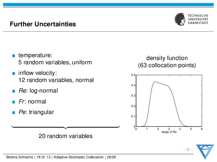
58. Further Uncertainties temperature: 5 random variables, uniform inflow velocity: 12 random variables, normal Re: log-normal Fr: normal Pe: triangular 20 random variables density function (63 collocation points) 0 1 2 3 4 5 6 0 0.1 0.2 0.3 0.4 0.5 range of Nu Bettina Schieche | 18.01.13 | Adaptive Stochastic Collocation | 26/28
59. Introduction of a Random (Rough) Surface bottom = 0 + 0.1 41 n=1 fn(x1)ξn small correlation length 41 random variables: uniform density dunction (211 collocation points) 2 2.5 3 3.5 0 1 2 3 4 5 6 range of Nu Bettina Schieche | 18.01.13 | Adaptive Stochastic Collocation | 27/28
60. Summary Summary: considered problems: PDEs with correlated random parameters exact calculation of moments for selected problems possible stochastic collocation as an efficient stochastic discretization tool Ongoing Research: analysis of commutator errors stochastic adjoint error estimation model order reduction Bettina Schieche | 18.01.13 | Adaptive Stochastic Collocation | 28/28
61. Konstruktion von d¨ unnbesetzten Gittern: Smolyak Algorithmus als Quadraturformel 1. geschachtelte Folge von 1d-Quadraturformeln: {Ui}i=1,2,... 2. definiere Tensorprodukt (Ui ⊗ Ul)(g) := j,k wj wk g(xj, xk ) 3. definiere Update-Formeln {∆i}i=1,2,... ∆1 := U1 ∆i := Ui − Ui−1 , i ≥ 2 4. Smolyak’s Formel A(k, M) := i1+...+iM ≤k+M ∆i1 ⊗ · · · ⊗ ∆iM Bettina Schieche | 18.01.13 | Adaptive Stochastic Collocation | 28/28
62. Wahl der rechten Seite des stochastischen adjungierten Problems A(u, ξ) = f(ξ) Q(u) = N(E[uq]) Q(u) − Q(uhξ ) ≈ N (E[uq hξ ])E[quq−1 hξ (u − uhξ )] = E[ qN (E[uq hξ ])uq−1 hξ rechte Seite von A∗(φ) (u − uhξ )] = E[ φ(A(u) =f −A(uhξ ))] = E[ φ(ξ)Res(uhξ )] Bettina Schieche | 18.01.13 | Adaptive Stochastic Collocation | 28/28
63. Modellreduktion des adjungierten Problems Proper Orthogonal Decomposition (POD) 1. Auswerten des adjungierten Problems in wenigen Kollokationspunkten: A∗(y(j))Φj = G, j = 1, . . . , P 2. Snapshot-Matrix S = (Φ1, · · · , ΦP) 3. Singul¨ arwertzerlegung von S → reduzierte Basis ϕ 4. Galerkin-Projektion auf ϕ: A∗ R (ξ)ΦR(ξ) = GR, dim(A∗ R ) dim(A∗) (1) 5. Auswerten von (1) in beliebig vielen Kollokationspunkten Bettina Schieche | 18.01.13 | Adaptive Stochastic Collocation | 28/28
64. Details zum Beweis A(a)S0(t)v = lim s→0+ Sa(s)S0(t)v − S0(t)v s = lim s→0+ S0(t)Sa(s)v − S0(t)v s = S0(t) lim s→0+ Sa(s)v − v s = S0(t)A(a)v mit Sa(s)S0(t)v = exp(A(a)s) exp(A(0)s)v = exp((A(a) + A(0))s) = exp(A(0)s) exp(A(a)s)v = S0(t)Sa(s)v Bettina Schieche | 18.01.13 | Adaptive Stochastic Collocation | 28/28