SOC 4650 & SOC 5650 - Lecture 08

Slides for Lecture 08 of the Saint Louis University Course Introduction to GIS. These slides introduce techniques for building geodatabases using ArcGIS Pro as well as additional cleaning and exporting data with RStudio.

Transcript

1. Clone (or pull if you’ve already cloned) the lecture-08 repository! Install the measurements package:
 install.packages(“measurements”) WELCOME! GETTING STARTED
2. COMBINING AND EXPORTING DATA INTRO TO GISC CHRISTOPHER PRENER, PH.D. SPRING 2020 WEEK 08 LECTURE 08
3. AGENDA INTRO TO GISC / WEEK 08 / LECTURE 08 1. Front Matter 2. Table Joins 3. Exporting Data 4. Geodatabases 5. Back Matter
4. 1 FRONT 
 MATTER
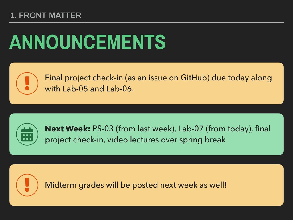
5. Final project check-in (as an issue on GitHub) due today along with Lab-05 and Lab-06. 1. FRONT MATTER ANNOUNCEMENTS Next Week: PS-03 (from last week), Lab-07 (from today), final project check-in, video lectures over spring break Midterm grades will be posted next week as well!
6. TABLE JOINS 2
7. 2. TABLE JOINS HIGH LEVEL WORKFLOW 1. Plan 2. Organize 3. Document 4. Execute FOR EACH
 STEP:
8. ▸ dplyr for data wrangling functions ▸ naniar for missing data analyses ▸ sf for working with spatial data 4. DATA WRANGLING PACKAGES
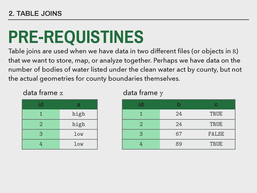
9. 2. TABLE JOINS PRE-REQUISTINES Table joins are used when we have data in two different files (or objects in R) that we want to store, map, or analyze together. Perhaps we have data on the number of bodies of water listed under the clean water act by county, but not the actual geometries for county boundaries themselves. id a 1 high 2 high 3 low 4 low id b c 1 24 TRUE 2 24 TRUE 3 67 FALSE 4 89 TRUE data frame x data frame y
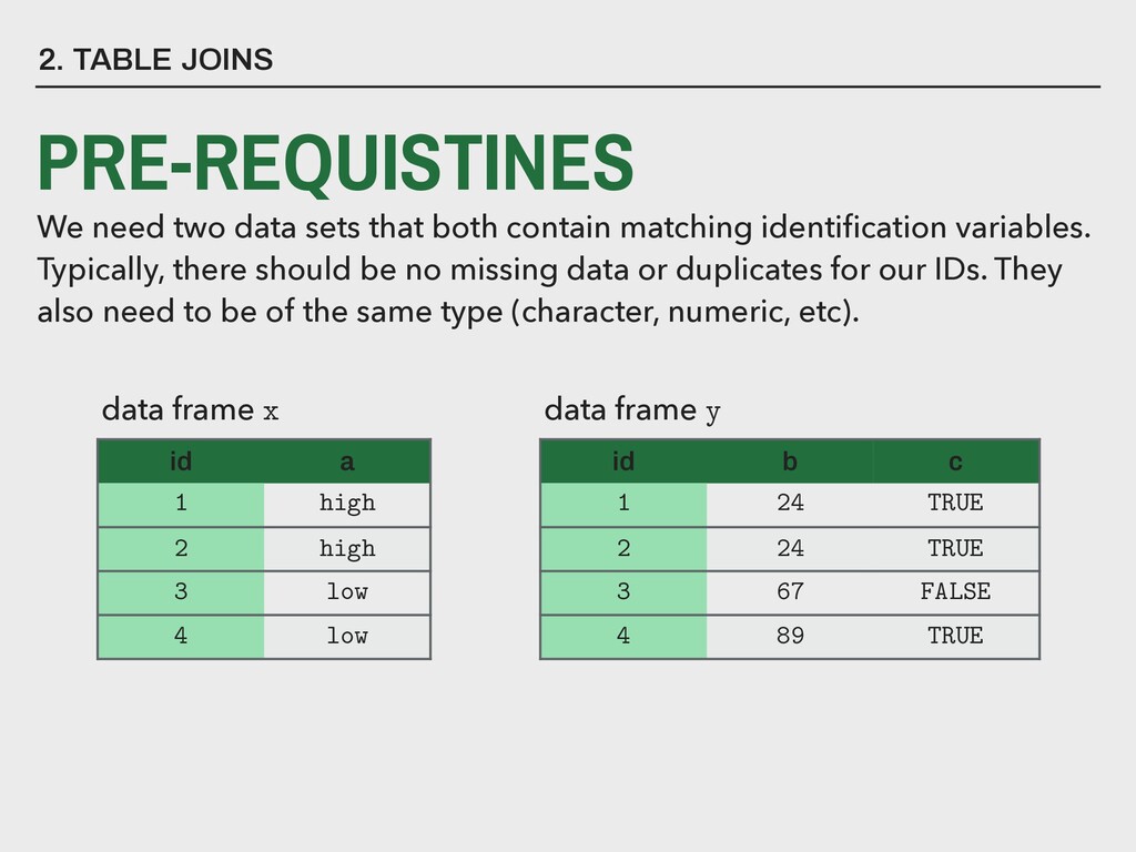
10. 2. TABLE JOINS PRE-REQUISTINES We need two data sets that both contain matching identification variables. Typically, there should be no missing data or duplicates for our IDs. They also need to be of the same type (character, numeric, etc). id a 1 high 2 high 3 low 4 low id b c 1 24 TRUE 2 24 TRUE 3 67 FALSE 4 89 TRUE data frame x data frame y
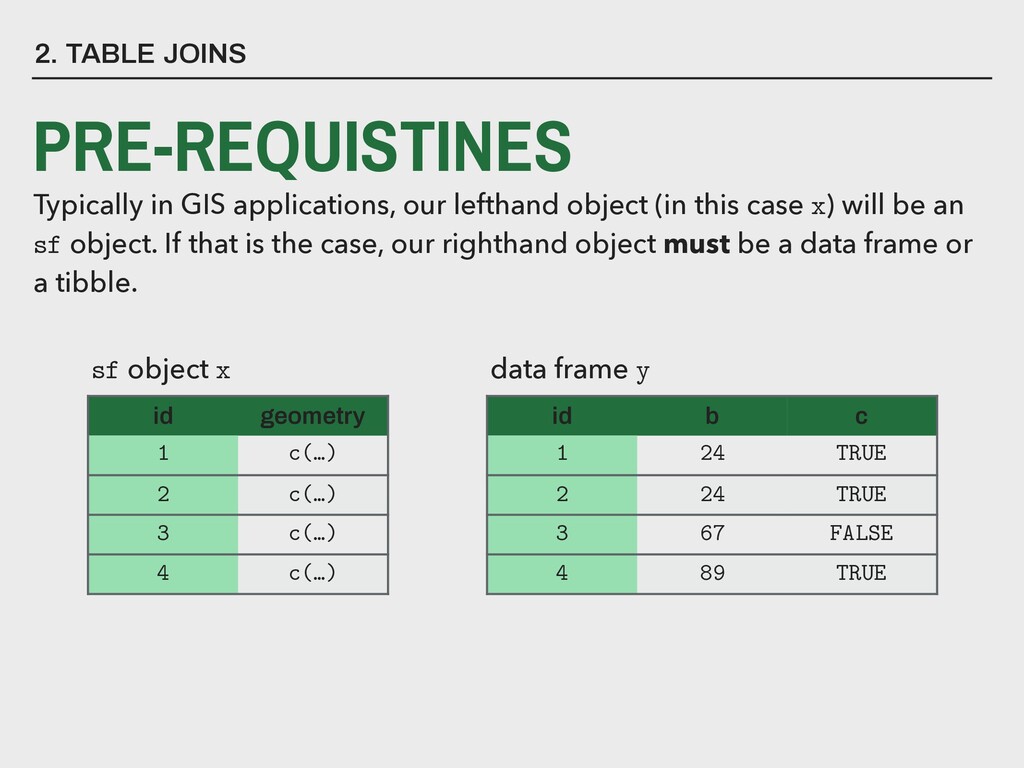
11. 2. TABLE JOINS PRE-REQUISTINES Typically in GIS applications, our lefthand object (in this case x) will be an sf object. If that is the case, our righthand object must be a data frame or a tibble. id geometry 1 c(…) 2 c(…) 3 c(…) 4 c(…) id b c 1 24 TRUE 2 24 TRUE 3 67 FALSE 4 89 TRUE sf object x data frame y
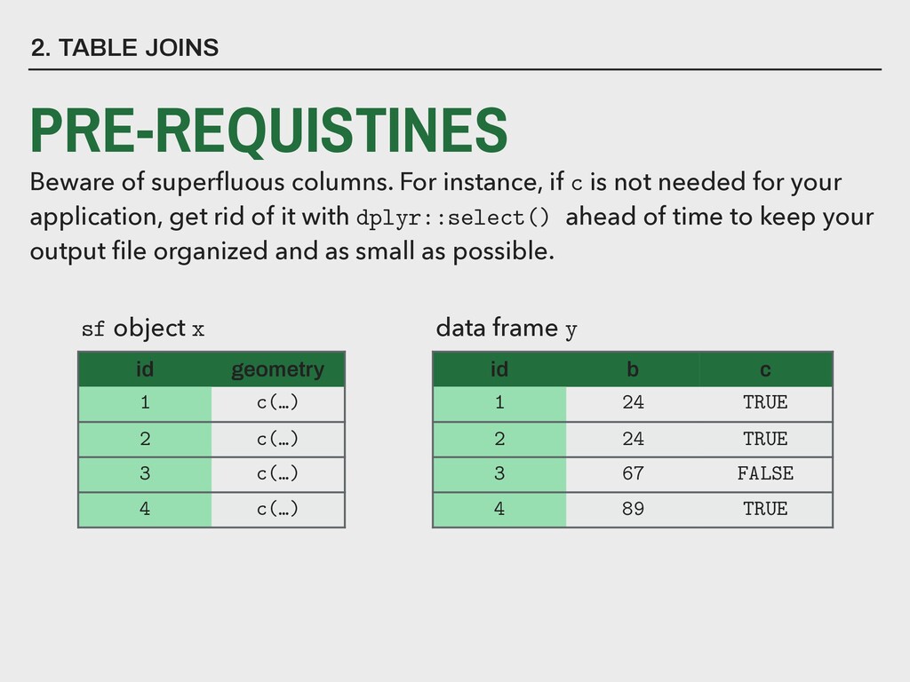
12. 2. TABLE JOINS PRE-REQUISTINES Beware of superfluous columns. For instance, if c is not needed for your application, get rid of it with dplyr::select() ahead of time to keep your output file organized and as small as possible. id geometry 1 c(…) 2 c(…) 3 c(…) 4 c(…) id b c 1 24 TRUE 2 24 TRUE 3 67 FALSE 4 89 TRUE sf object x data frame y
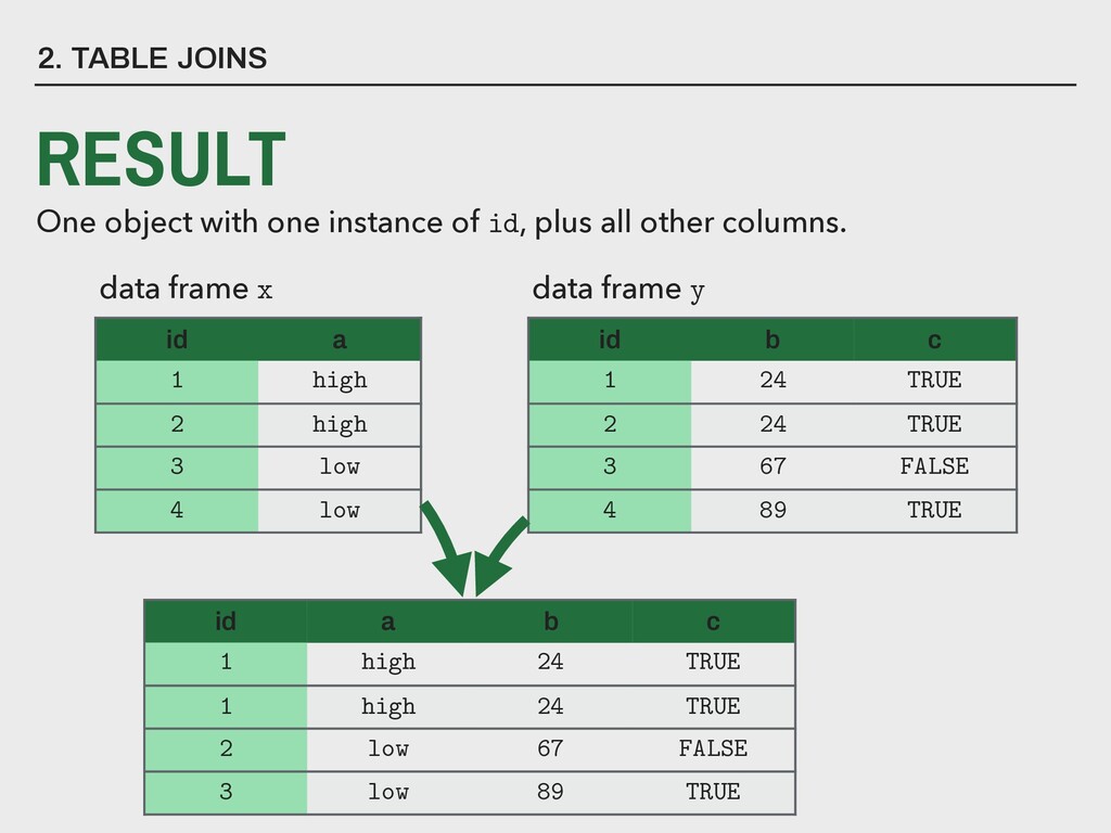
13. 2. TABLE JOINS RESULT One object with one instance of id, plus all other columns. id a 1 high 2 high 3 low 4 low id b c 1 24 TRUE 2 24 TRUE 3 67 FALSE 4 89 TRUE data frame x data frame y id a b c 1 high 24 TRUE 1 high 24 TRUE 2 low 67 FALSE 3 low 89 TRUE
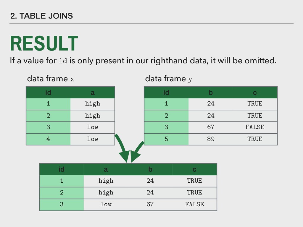
14. 2. TABLE JOINS RESULT If a value for id is only present in our righthand data, it will be omitted. id a 1 high 2 high 3 low 4 low id b c 1 24 TRUE 2 24 TRUE 3 67 FALSE 5 89 TRUE data frame x data frame y id a b c 1 high 24 TRUE 2 high 24 TRUE 3 low 67 FALSE
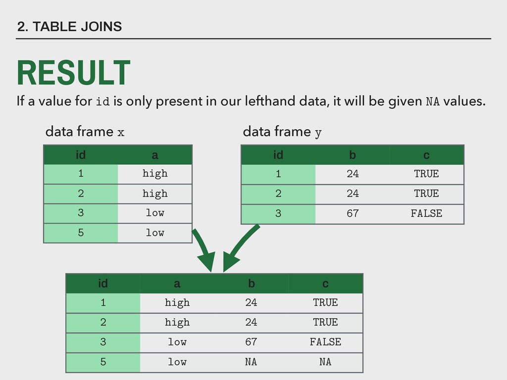
15. 2. TABLE JOINS RESULT If a value for id is only present in our lefthand data, it will be given NA values. id a 1 high 2 high 3 low 5 low id b c 1 24 TRUE 2 24 TRUE 3 67 FALSE data frame x data frame y id a b c 1 high 24 TRUE 2 high 24 TRUE 3 low 67 FALSE 5 low NA NA
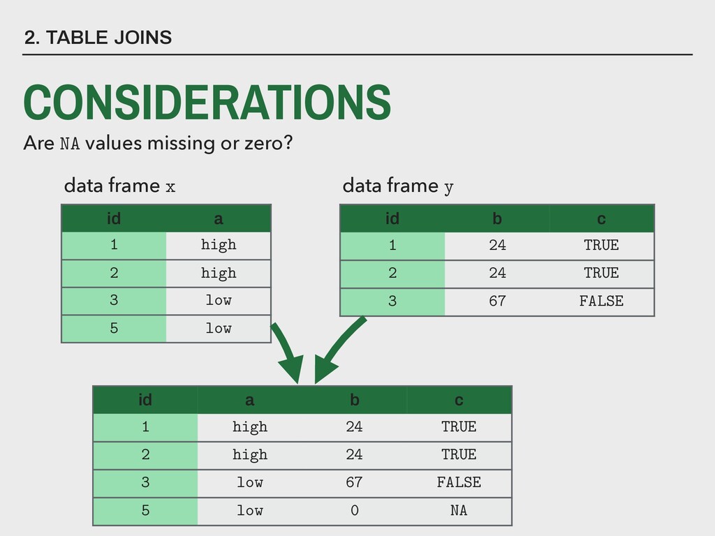
16. 2. TABLE JOINS CONSIDERATIONS Are NA values missing or zero? id a 1 high 2 high 3 low 5 low id b c 1 24 TRUE 2 24 TRUE 3 67 FALSE data frame x data frame y id a b c 1 high 24 TRUE 2 high 24 TRUE 3 low 67 FALSE 5 low 0 NA
17. EXPORTING DATA 3
18. ▸ dplyr for data wrangling functions ▸ readr for writing tabular data ▸ sf for preparing columns and writing spatial data 4. DATA WRANGLING PACKAGES
19. ▸ .csv for any tabular data applications ▸ .shp for 99.9% of spatial data applications ▸ .geoJSON for map previews on github.com 4. DATA WRANGLING FORMATS
20. GEODATABASES 4
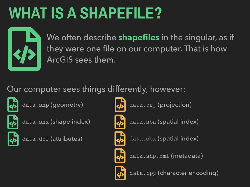
21. WHAT IS A SHAPEFILE? We often describe shapefiles in the singular, as if they were one file on our computer. That is how ArcGIS sees them. Our computer sees things differently, however: data.shp (geometry) data.shx (shape index) data.dbf (attributes) data.sbn (spatial index) data.sbx (spatial index) data.shp.xml (metadata) data.cpg (character encoding) data.prj (projection)
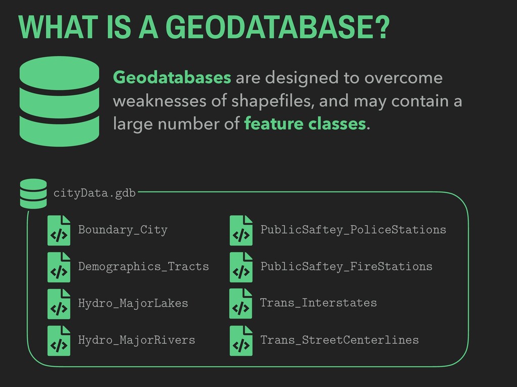
22. WHAT IS A GEODATABASE? Geodatabases are designed to overcome weaknesses of shapefiles, and may contain a large number of feature classes. cityData.gdb Boundary_City Demographics_Tracts Hydro_MajorLakes Hydro_MajorRivers PublicSaftey_PoliceStations PublicSaftey_FireStations Trans_Interstates Trans_StreetCenterlines
23. 5 BACK 
 MATTER
24. AGENDA REVIEW 5. BACK MATTER 2. Table Joins 3. Exporting Data 4. Geodatabases
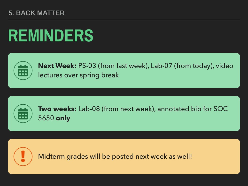
25. Two weeks: Lab-08 (from next week), annotated bib for SOC 5650 only Next Week: PS-03 (from last week), Lab-07 (from today), video lectures over spring break REMINDERS 5. BACK MATTER Midterm grades will be posted next week as well!