$30 off During Our Annual Pro Sale. View Details »

Python and PostgreSQL: Let's Work Together! | PyConFr 2018 | Dimitri Fontaine

Citus Data
October 07, 2018

Python and PostgreSQL: Let's Work Together! | PyConFr 2018 | Dimitri Fontaine

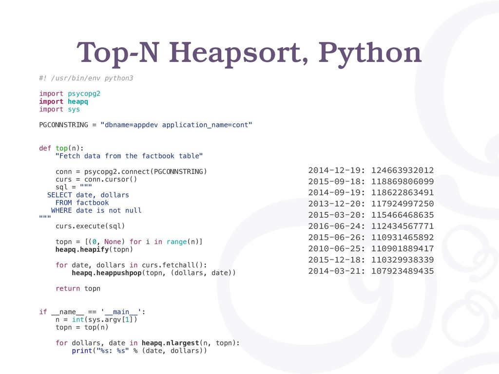
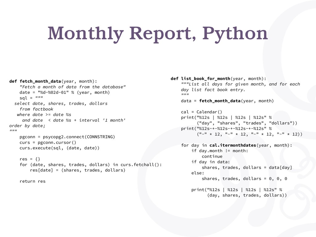
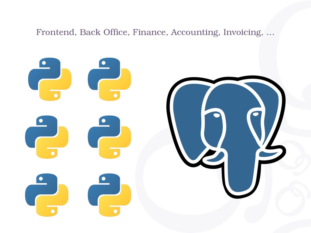
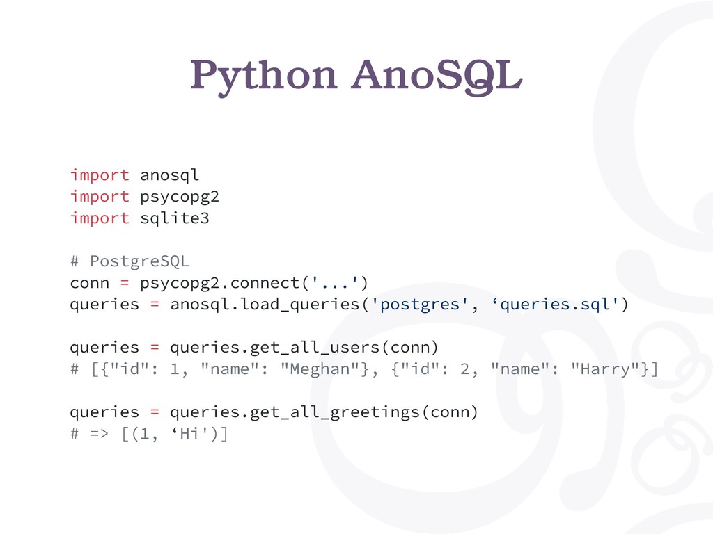
Python is often used to maintain application backends. When the backend should implement user oriented workflows, it may rely on a RDBMS component to take care of the system's integrity.

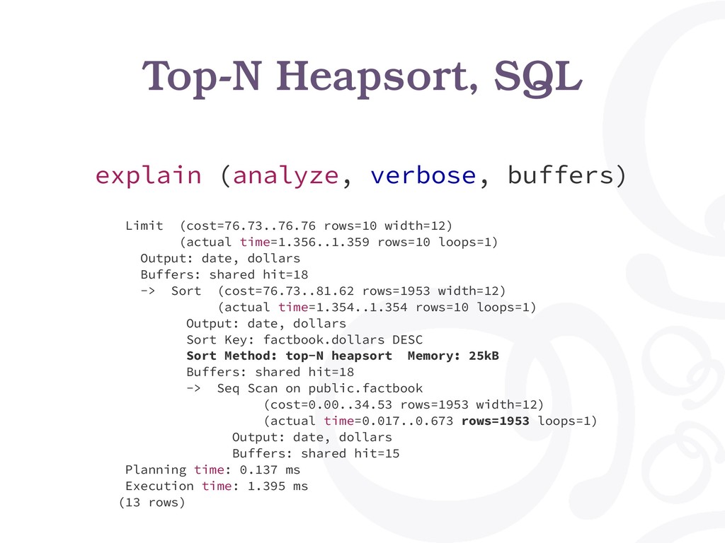
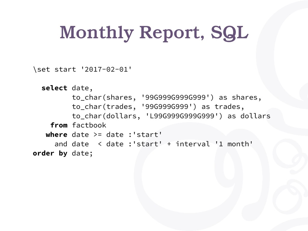
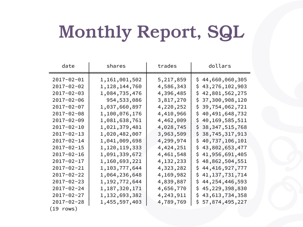
PostgreSQL is the world's most advanced open source relational database, and is very good at taking care of your system's integrity. PostgreSQL also comes with a ton of data processing power, and in many cases a simple enough SQL statement may replace hundreds of lines of code written in Python.

In this talk, we learn advanced SQL techniques and how to reason about which part of the backend code should be done in the database, and which parf of the backend code is so easier to write as a SQL query.
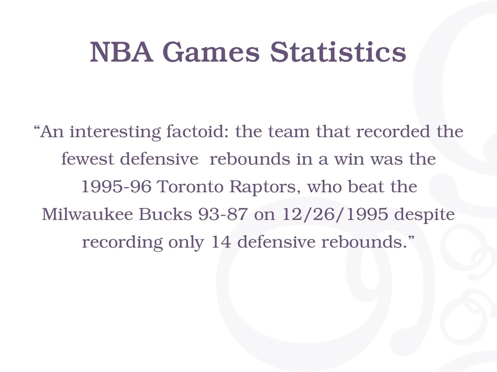
Citus Data

October 07, 2018
Tweet

More Decks by Citus Data

Other Decks in Technology

Transcript

  1. Python and PostgreSQL
    Let’s work together!
    Dimitri Fontaine
    Citus Data
    P Y C O N F R , L I L L E | O C T O B E R 7 , 2 0 1 8

    View Slide

  2. Python
    U S E R S I N C E 1 . 5 . 2

    View Slide

  3. PostgreSQL
    P O S T G R E S Q L M A J O R C O N T R I B U T O R

    View Slide

  4. Citus Data
    C U R R E N T L Y W O R K I N G A T

    View Slide

  5. Mastering
    PostgreSQL
    In Application
    Development
    https://masteringpostgresql.com

    View Slide

  6. Mastering
    PostgreSQL
    In Application
    Development
    -15%
    “pyconfr2018”
    https://masteringpostgresql.com

    View Slide

  7. pgloader.io

    View Slide

  8. Let’s work together!

    View Slide

  9. Why use a RDBMS?

    View Slide

  10. Concurrency & Isolation
    R E L A T I O N A L D A T A B A S E M A N A G E M E N T S Y S T E M

    View Slide

  11. ACID
    A relational database management system guarantees
    consistency of a system as a whole while allowing concurrent
    access (read and write) to a single data set.
    • Atomic
    • Consistent
    • Isolated
    • Durable
    Dimitri Fontaine (CitusData) Data Modeling, Normalization and Denormalization March 13, 2018

    View Slide

  12. Atomic
    Dimitri Fontaine (CitusData) Data Modeling, Normalization and Denormalization March 13, 2018
    ROLLBACK;

    View Slide

  13. Consistent
    Dimitri Fontaine (CitusData) Data Modeling, Normalization and Denormalization March 13, 2018
    • Data types
    • Constraints
    check, not null,
    pkey, fkey
    • Relations
    • SQL
    • Schema
    create table foo
    (
    id int,
    f1 text
    );

    View Slide

  14. Isolated
    Dimitri Fontaine (CitusData) Data Modeling, Normalization and Denormalization March 13, 2018
    $ pg_dump

    View Slide

  15. Durable
    Dimitri Fontaine (CitusData) Data Modeling, Normalization and Denormalization March 13, 2018

    View Slide

  16. Software Architecture

    View Slide

  17. Application (user workflow) and PostgreSQL (system rules)

    View Slide

  18. Rule 5. Data dominates.
    R O B P I K E , N O T E S O N P R O G R A M M I N G I N C
    “If you’ve chosen the right data structures and
    organized things well, the algorithms will
    almost always be self-evident. Data structures,
    not algorithms, are central to programming.”
    (Brooks p. 102)

    View Slide

  19. New York Stock Exchange

    View Slide

  20. Daily NYSE Group Volume in
    NYSE Listed, 2017
    2010 1/4/2010 1,425,504,460 4,628,115 $38,495,460,645
    2010 1/5/2010 1,754,011,750 5,394,016 $43,932,043,406
    2010 1/6/2010 1,655,507,953 5,494,460 $43,816,749,660
    2010 1/7/2010 1,797,810,789 5,674,297 $44,104,237,184
    create table factbook
    (
    year int,
    date date,
    shares text,
    trades text,
    dollars text
    );
    \copy factbook from 'factbook.csv' with delimiter E'\t' null ''

    View Slide

  21. Daily NYSE Group Volume in
    NYSE Listed, 2017
    alter table factbook
    alter shares
    type bigint
    using replace(shares, ',', '')::bigint,
    alter trades
    type bigint
    using replace(trades, ',', '')::bigint,
    alter dollars
    type bigint
    using substring(replace(dollars, ',', '') from 2)::numeric;

    View Slide

  22. SQL and Algorithms

    View Slide

  23. Top-N Heapsort, Python
    #! /usr/bin/env python3
    import psycopg2
    import heapq
    import sys
    PGCONNSTRING = "dbname=appdev application_name=cont"
    def top(n):
    "Fetch data from the factbook table"
    conn = psycopg2.connect(PGCONNSTRING)
    curs = conn.cursor()
    sql = """
    SELECT date, dollars
    FROM factbook
    WHERE date is not null
    """
    curs.execute(sql)
    topn = [(0, None) for i in range(n)]
    heapq.heapify(topn)
    for date, dollars in curs.fetchall():
    heapq.heappushpop(topn, (dollars, date))
    return topn
    if __name__ == '__main__':
    n = int(sys.argv[1])
    topn = top(n)
    for dollars, date in heapq.nlargest(n, topn):
    print("%s: %s" % (date, dollars))
    2014-12-19: 124663932012
    2015-09-18: 118869806099
    2014-09-19: 118622863491
    2013-12-20: 117924997250
    2015-03-20: 115466468635
    2016-06-24: 112434567771
    2015-06-26: 110931465892
    2010-06-25: 110901889417
    2015-12-18: 110329938339
    2014-03-21: 107923489435

    View Slide

  24. select date, dollars
    from factbook
    order by dollars desc
    limit 10;
    Top-N Heapsort, SQL
    date │ dollars
    ════════════╪══════════════
    2014-12-19 │ 124663932012
    2015-09-18 │ 118869806099
    2014-09-19 │ 118622863491
    2013-12-20 │ 117924997250
    2015-03-20 │ 115466468635
    2016-06-24 │ 112434567771
    2015-06-26 │ 110931465892
    2010-06-25 │ 110901889417
    2015-12-18 │ 110329938339
    2014-03-21 │ 107923489435
    (10 rows)

    View Slide

  25. Limit (cost=76.73..76.76 rows=10 width=12)
    (actual time=1.356..1.359 rows=10 loops=1)
    Output: date, dollars
    Buffers: shared hit=18
    -> Sort (cost=76.73..81.62 rows=1953 width=12)
    (actual time=1.354..1.354 rows=10 loops=1)
    Output: date, dollars
    Sort Key: factbook.dollars DESC
    Sort Method: top-N heapsort Memory: 25kB
    Buffers: shared hit=18
    -> Seq Scan on public.factbook
    (cost=0.00..34.53 rows=1953 width=12)
    (actual time=0.017..0.673 rows=1953 loops=1)
    Output: date, dollars
    Buffers: shared hit=15
    Planning time: 0.137 ms
    Execution time: 1.395 ms
    (13 rows)
    Top-N Heapsort, SQL
    explain (analyze, verbose, buffers)

    View Slide

  26. Monthly Reports

    View Slide

  27. Monthly Report, SQL
    \set start '2017-02-01'
    select date,
    to_char(shares, '99G999G999G999') as shares,
    to_char(trades, '99G999G999') as trades,
    to_char(dollars, 'L99G999G999G999') as dollars
    from factbook
    where date >= date :'start'
    and date < date :'start' + interval '1 month'
    order by date;

    View Slide

  28. Monthly Report, SQL
    date │ shares │ trades │ dollars
    ════════════╪═════════════════╪═════════════╪══════════════════
    2017-02-01 │ 1,161,001,502 │ 5,217,859 │ $ 44,660,060,305
    2017-02-02 │ 1,128,144,760 │ 4,586,343 │ $ 43,276,102,903
    2017-02-03 │ 1,084,735,476 │ 4,396,485 │ $ 42,801,562,275
    2017-02-06 │ 954,533,086 │ 3,817,270 │ $ 37,300,908,120
    2017-02-07 │ 1,037,660,897 │ 4,220,252 │ $ 39,754,062,721
    2017-02-08 │ 1,100,076,176 │ 4,410,966 │ $ 40,491,648,732
    2017-02-09 │ 1,081,638,761 │ 4,462,009 │ $ 40,169,585,511
    2017-02-10 │ 1,021,379,481 │ 4,028,745 │ $ 38,347,515,768
    2017-02-13 │ 1,020,482,007 │ 3,963,509 │ $ 38,745,317,913
    2017-02-14 │ 1,041,009,698 │ 4,299,974 │ $ 40,737,106,101
    2017-02-15 │ 1,120,119,333 │ 4,424,251 │ $ 43,802,653,477
    2017-02-16 │ 1,091,339,672 │ 4,461,548 │ $ 41,956,691,405
    2017-02-17 │ 1,160,693,221 │ 4,132,233 │ $ 48,862,504,551
    2017-02-21 │ 1,103,777,644 │ 4,323,282 │ $ 44,416,927,777
    2017-02-22 │ 1,064,236,648 │ 4,169,982 │ $ 41,137,731,714
    2017-02-23 │ 1,192,772,644 │ 4,839,887 │ $ 44,254,446,593
    2017-02-24 │ 1,187,320,171 │ 4,656,770 │ $ 45,229,398,830
    2017-02-27 │ 1,132,693,382 │ 4,243,911 │ $ 43,613,734,358
    2017-02-28 │ 1,455,597,403 │ 4,789,769 │ $ 57,874,495,227
    (19 rows)

    View Slide

  29. Monthly Report, Python
    def fetch_month_data(year, month):
    "Fetch a month of data from the database"
    date = "%d-%02d-01" % (year, month)
    sql = """
    select date, shares, trades, dollars
    from factbook
    where date >= date %s
    and date < date %s + interval '1 month'
    order by date;
    """
    pgconn = psycopg2.connect(CONNSTRING)
    curs = pgconn.cursor()
    curs.execute(sql, (date, date))
    res = {}
    for (date, shares, trades, dollars) in curs.fetchall():
    res[date] = (shares, trades, dollars)
    return res
    def list_book_for_month(year, month):
    """List all days for given month, and for each
    day list fact book entry.
    """
    data = fetch_month_data(year, month)
    cal = Calendar()
    print("%12s | %12s | %12s | %12s" %
    ("day", "shares", "trades", "dollars"))
    print("%12s-+-%12s-+-%12s-+-%12s" %
    ("-" * 12, "-" * 12, "-" * 12, "-" * 12))
    for day in cal.itermonthdates(year, month):
    if day.month != month:
    continue
    if day in data:
    shares, trades, dollars = data[day]
    else:
    shares, trades, dollars = 0, 0, 0
    print("%12s | %12s | %12s | %12s" %
    (day, shares, trades, dollars))

    View Slide

  30. $ ./factbook-month.py 2017 2
    day | shares | trades | dollars
    -------------+--------------+--------------+-------------
    2017-02-01 | 1161001502 | 5217859 | 44660060305
    2017-02-02 | 1128144760 | 4586343 | 43276102903
    2017-02-03 | 1084735476 | 4396485 | 42801562275
    2017-02-04 | 0 | 0 | 0
    2017-02-05 | 0 | 0 | 0
    2017-02-06 | 954533086 | 3817270 | 37300908120
    2017-02-07 | 1037660897 | 4220252 | 39754062721
    2017-02-08 | 1100076176 | 4410966 | 40491648732
    2017-02-09 | 1081638761 | 4462009 | 40169585511
    2017-02-10 | 1021379481 | 4028745 | 38347515768
    2017-02-11 | 0 | 0 | 0
    2017-02-12 | 0 | 0 | 0
    2017-02-13 | 1020482007 | 3963509 | 38745317913
    2017-02-14 | 1041009698 | 4299974 | 40737106101
    2017-02-15 | 1120119333 | 4424251 | 43802653477
    2017-02-16 | 1091339672 | 4461548 | 41956691405
    2017-02-17 | 1160693221 | 4132233 | 48862504551
    2017-02-18 | 0 | 0 | 0
    2017-02-19 | 0 | 0 | 0
    2017-02-20 | 0 | 0 | 0
    2017-02-21 | 1103777644 | 4323282 | 44416927777
    2017-02-22 | 1064236648 | 4169982 | 41137731714
    2017-02-23 | 1192772644 | 4839887 | 44254446593
    2017-02-24 | 1187320171 | 4656770 | 45229398830
    2017-02-25 | 0 | 0 | 0
    2017-02-26 | 0 | 0 | 0
    2017-02-27 | 1132693382 | 4243911 | 43613734358
    2017-02-28 | 1455597403 | 4789769 | 57874495227
    Monthly Report, Python

    View Slide

  31. Where is that code used?

    View Slide

  32. Frontend, Back Office, Finance, Accounting, Invoicing, …

    View Slide

  33. Days with no activity, SQL

    View Slide

  34. Monthly Report, Fixed, SQL
    select cast(calendar.entry as date) as date,
    coalesce(shares, 0) as shares,
    coalesce(trades, 0) as trades,
    to_char(
    coalesce(dollars, 0),
    'L99G999G999G999'
    ) as dollars
    from /*
    * Generate the target month's calendar then LEFT JOIN
    * each day against the factbook dataset, so as to have
    * every day in the result set, whether or not we have a
    * book entry for the day.
    */
    generate_series(date :'start',
    date :'start' + interval '1 month'
    - interval '1 day',
    interval '1 day'
    )
    as calendar(entry)
    left join factbook
    on factbook.date = calendar.entry
    order by date;

    View Slide

  35. date │ shares │ trades │ dollars
    ════════════╪════════════╪═════════╪══════════════════
    2017-02-01 │ 1161001502 │ 5217859 │ $ 44,660,060,305
    2017-02-02 │ 1128144760 │ 4586343 │ $ 43,276,102,903
    2017-02-03 │ 1084735476 │ 4396485 │ $ 42,801,562,275
    2017-02-04 │ 0 │ 0 │ $ 0
    2017-02-05 │ 0 │ 0 │ $ 0
    2017-02-06 │ 954533086 │ 3817270 │ $ 37,300,908,120
    2017-02-07 │ 1037660897 │ 4220252 │ $ 39,754,062,721
    2017-02-08 │ 1100076176 │ 4410966 │ $ 40,491,648,732
    2017-02-09 │ 1081638761 │ 4462009 │ $ 40,169,585,511
    2017-02-10 │ 1021379481 │ 4028745 │ $ 38,347,515,768
    2017-02-11 │ 0 │ 0 │ $ 0
    2017-02-12 │ 0 │ 0 │ $ 0
    2017-02-13 │ 1020482007 │ 3963509 │ $ 38,745,317,913
    2017-02-14 │ 1041009698 │ 4299974 │ $ 40,737,106,101
    2017-02-15 │ 1120119333 │ 4424251 │ $ 43,802,653,477
    2017-02-16 │ 1091339672 │ 4461548 │ $ 41,956,691,405
    2017-02-17 │ 1160693221 │ 4132233 │ $ 48,862,504,551
    2017-02-18 │ 0 │ 0 │ $ 0
    2017-02-19 │ 0 │ 0 │ $ 0
    2017-02-20 │ 0 │ 0 │ $ 0
    2017-02-21 │ 1103777644 │ 4323282 │ $ 44,416,927,777
    2017-02-22 │ 1064236648 │ 4169982 │ $ 41,137,731,714
    2017-02-23 │ 1192772644 │ 4839887 │ $ 44,254,446,593
    2017-02-24 │ 1187320171 │ 4656770 │ $ 45,229,398,830
    2017-02-25 │ 0 │ 0 │ $ 0
    2017-02-26 │ 0 │ 0 │ $ 0
    2017-02-27 │ 1132693382 │ 4243911 │ $ 43,613,734,358
    2017-02-28 │ 1455597403 │ 4789769 │ $ 57,874,495,227
    (28 rows)
    Monthly Report, Fixed, SQL

    View Slide

  36. Marketing dept wants
    Week on Week Evolution

    View Slide

  37. date │ day │ dollars │ WoW %
    ════════════╪═════╪══════════════════╪════════
    2017-02-01 │ Wed │ $ 44,660,060,305 │ -2.21
    2017-02-02 │ Thu │ $ 43,276,102,903 │ 1.71
    2017-02-03 │ Fri │ $ 42,801,562,275 │ 10.86
    2017-02-04 │ Sat │ $ 0 │ ¤
    2017-02-05 │ Sun │ $ 0 │ ¤
    2017-02-06 │ Mon │ $ 37,300,908,120 │ -9.64
    2017-02-07 │ Tue │ $ 39,754,062,721 │ -37.41
    2017-02-08 │ Wed │ $ 40,491,648,732 │ -10.29
    2017-02-09 │ Thu │ $ 40,169,585,511 │ -7.73
    2017-02-10 │ Fri │ $ 38,347,515,768 │ -11.61
    2017-02-11 │ Sat │ $ 0 │ ¤
    2017-02-12 │ Sun │ $ 0 │ ¤
    2017-02-13 │ Mon │ $ 38,745,317,913 │ 3.73
    2017-02-14 │ Tue │ $ 40,737,106,101 │ 2.41
    2017-02-15 │ Wed │ $ 43,802,653,477 │ 7.56
    2017-02-16 │ Thu │ $ 41,956,691,405 │ 4.26
    2017-02-17 │ Fri │ $ 48,862,504,551 │ 21.52
    2017-02-18 │ Sat │ $ 0 │ ¤
    2017-02-19 │ Sun │ $ 0 │ ¤
    2017-02-20 │ Mon │ $ 0 │ ¤
    2017-02-21 │ Tue │ $ 44,416,927,777 │ 8.28
    2017-02-22 │ Wed │ $ 41,137,731,714 │ -6.48
    2017-02-23 │ Thu │ $ 44,254,446,593 │ 5.19
    2017-02-24 │ Fri │ $ 45,229,398,830 │ -8.03
    2017-02-25 │ Sat │ $ 0 │ ¤
    2017-02-26 │ Sun │ $ 0 │ ¤
    2017-02-27 │ Mon │ $ 43,613,734,358 │ ¤
    2017-02-28 │ Tue │ $ 57,874,495,227 │ 23.25
    (28 rows)
    Monthly Report, WoW%, SQL

    View Slide

  38. View Slide

  39. Monthly Report, WoW%, SQL
    with computed_data as
    (
    select cast(date as date) as date,
    to_char(date, 'Dy') as day,
    coalesce(dollars, 0) as dollars,
    lag(dollars, 1)
    over(
    partition by extract('isodow' from date)
    order by date
    )
    as last_week_dollars
    from /*
    * Generate the month calendar, plus a week
    * before so that we have values to compare
    * dollars against even for the first week
    * of the month.
    */
    generate_series(date :'start' - interval '1 week',
    date :'start' + interval '1 month'
    - interval '1 day',
    interval '1 day'
    )
    as calendar(date)
    left join factbook using(date)
    )
    select date, day,
    to_char(
    coalesce(dollars, 0),
    'L99G999G999G999'
    ) as dollars,
    case when dollars is not null
    and dollars <> 0
    then round( 100.0
    * (dollars - last_week_dollars)
    / dollars
    , 2)
    end
    as "WoW %"
    from computed_data
    where date >= date :'start'
    order by date;

    View Slide

  40. Monthly Report, WoW%, SQL
    with computed_data as
    (
    select cast(date as date) as date,
    to_char(date, 'Dy') as day,
    coalesce(dollars, 0) as dollars,
    lag(dollars, 1)
    over(
    partition by extract('isodow' from date)
    order by date
    )
    as last_week_dollars
    from /*
    * Generate the month calendar, plus a week
    * before so that we have values to compare
    * dollars against even for the first week
    * of the month.
    */
    generate_series(date :'start' - interval '1 week',
    date :'start' + interval '1 month'
    - interval '1 day',
    interval '1 day'
    )
    as calendar(date)
    left join factbook using(date)
    )
    select date, day,
    to_char(
    coalesce(dollars, 0),
    'L99G999G999G999'
    ) as dollars,
    case when dollars is not null
    and dollars <> 0
    then round( 100.0
    * (dollars - last_week_dollars)
    / dollars
    , 2)
    end
    as "WoW %"
    from computed_data
    where date >= date :'start'
    order by date;
    Window Function, SQL’92

    View Slide

  41. date │ day │ dollars │ WoW %
    ════════════╪═════╪══════════════════╪════════
    2017-02-01 │ Wed │ $ 44,660,060,305 │ -2.21
    2017-02-02 │ Thu │ $ 43,276,102,903 │ 1.71
    2017-02-03 │ Fri │ $ 42,801,562,275 │ 10.86
    2017-02-04 │ Sat │ $ 0 │ ¤
    2017-02-05 │ Sun │ $ 0 │ ¤
    2017-02-06 │ Mon │ $ 37,300,908,120 │ -9.64
    2017-02-07 │ Tue │ $ 39,754,062,721 │ -37.41
    2017-02-08 │ Wed │ $ 40,491,648,732 │ -10.29
    2017-02-09 │ Thu │ $ 40,169,585,511 │ -7.73
    2017-02-10 │ Fri │ $ 38,347,515,768 │ -11.61
    2017-02-11 │ Sat │ $ 0 │ ¤
    2017-02-12 │ Sun │ $ 0 │ ¤
    2017-02-13 │ Mon │ $ 38,745,317,913 │ 3.73
    2017-02-14 │ Tue │ $ 40,737,106,101 │ 2.41
    2017-02-15 │ Wed │ $ 43,802,653,477 │ 7.56
    2017-02-16 │ Thu │ $ 41,956,691,405 │ 4.26
    2017-02-17 │ Fri │ $ 48,862,504,551 │ 21.52
    2017-02-18 │ Sat │ $ 0 │ ¤
    2017-02-19 │ Sun │ $ 0 │ ¤
    2017-02-20 │ Mon │ $ 0 │ ¤
    2017-02-21 │ Tue │ $ 44,416,927,777 │ 8.28
    2017-02-22 │ Wed │ $ 41,137,731,714 │ -6.48
    2017-02-23 │ Thu │ $ 44,254,446,593 │ 5.19
    2017-02-24 │ Fri │ $ 45,229,398,830 │ -8.03
    2017-02-25 │ Sat │ $ 0 │ ¤
    2017-02-26 │ Sun │ $ 0 │ ¤
    2017-02-27 │ Mon │ $ 43,613,734,358 │ ¤
    2017-02-28 │ Tue │ $ 57,874,495,227 │ 23.25
    (28 rows)
    Monthly Report, WoW%, SQL

    View Slide

  42. The SQL Standard
    SQL:2016

    View Slide

  43. Thinking in SQL
    •Structured Query Language
    •Declarative Programming Language
    •Relational Model
    •Unix: everything is a file
    •Java: everything is an object
    •Python: packages, modules, classes, methods
    •SQL: relations

    View Slide

  44. SQL Relations
    •SELECT describes the type of the relation
    •Named a projection operator
    •Defines SQL Query Attribute domains
    •FROM introduces base relations
    •Relational Operators compute new relations
    •INNER JOIN
    •OUTER JOIN
    •LATERAL JOIN
    •set operators: UNION, EXECPT, INTERSECT

    View Slide

  45. SQL Relations
    with decades as
    (
    select extract('year' from date_trunc('decade', date)) as decade
    from races
    group by decade
    )
    select decade,
    rank() over(partition by decade order by wins desc) as rank,
    forename, surname, wins
    from decades
    left join lateral
    (
    select code, forename, surname, count(*) as wins
    from drivers
    join results
    on results.driverid = drivers.driverid
    and results.position = 1
    join races using(raceid)
    where extract('year' from date_trunc('decade', races.date))
    = decades.decade
    group by decades.decade, drivers.driverid
    order by wins desc
    limit 3
    )
    as winners on true
    order by decade asc, wins desc;

    View Slide

  46. Top-3 Pilots by decade
    decade │ rank │ forename │ surname │ wins
    ════════╪══════╪═══════════╪════════════╪══════
    1950 │ 1 │ Juan │ Fangio │ 24
    1950 │ 2 │ Alberto │ Ascari │ 13
    1950 │ 3 │ Stirling │ Moss │ 12
    1960 │ 1 │ Jim │ Clark │ 25
    1960 │ 2 │ Graham │ Hill │ 14
    1960 │ 3 │ Jack │ Brabham │ 11
    1970 │ 1 │ Niki │ Lauda │ 17
    1970 │ 2 │ Jackie │ Stewart │ 16
    1970 │ 3 │ Emerson │ Fittipaldi │ 14
    1980 │ 1 │ Alain │ Prost │ 39
    1980 │ 2 │ Nelson │ Piquet │ 20
    1980 │ 2 │ Ayrton │ Senna │ 20
    1990 │ 1 │ Michael │ Schumacher │ 35
    1990 │ 2 │ Damon │ Hill │ 22
    1990 │ 3 │ Ayrton │ Senna │ 21
    2000 │ 1 │ Michael │ Schumacher │ 56
    2000 │ 2 │ Fernando │ Alonso │ 21
    2000 │ 3 │ Kimi │ Räikkönen │ 18
    2010 │ 1 │ Lewis │ Hamilton │ 45
    2010 │ 2 │ Sebastian │ Vettel │ 40
    2010 │ 3 │ Nico │ Rosberg │ 23
    (21 rows)

    View Slide

  47. SQL is Code

    View Slide

  48. SQL & Developer Tooling
    with computed_data as
    (
    select cast(date as date) as date,
    to_char(date, 'Dy') as day,
    coalesce(dollars, 0) as dollars,
    lag(dollars, 1)
    over(
    partition by extract('isodow' from date)
    order by date
    )
    as last_week_dollars
    from /*
    * Generate the month calendar, plus a week before
    * so that we have values to compare dollars against
    * even for the first week of the month.
    */
    generate_series(date :'start' - interval '1 week',
    date :'start' + interval '1 month'
    - interval '1 day',
    interval '1 day'
    )
    as calendar(date)
    left join factbook using(date)
    )
    select date, day,
    to_char(
    coalesce(dollars, 0),
    'L99G999G999G999'
    ) as dollars,
    case when dollars is not null
    and dollars <> 0
    then round( 100.0
    * (dollars - last_week_dollars)
    / dollars
    , 2)
    end
    as "WoW %"
    from computed_data
    where date >= date :'start'
    order by date;
    • Code Integration
    • SQL Queries in .sql files
    • Parameters
    • Result Set To Objects
    • A Result Set is a Relation
    • Testing
    • Unit Testing
    • Regression Testing

    View Slide

  49. Python AnoSQL
    $ cat queries.sql
    -- name: get-all-greetings
    -- Get all the greetings in the database
    SELECT * FROM greetings;
    -- name: $select-users
    -- Get all the users from the database,
    -- and return it as a dict
    SELECT * FROM USERS;

    View Slide

  50. import anosql
    import psycopg2
    import sqlite3
    # PostgreSQL
    conn = psycopg2.connect('...')
    queries = anosql.load_queries('postgres', ‘queries.sql')
    queries = queries.get_all_users(conn)
    # [{"id": 1, "name": "Meghan"}, {"id": 2, "name": "Harry"}]
    queries = queries.get_all_greetings(conn)
    # => [(1, ‘Hi')]
    Python AnoSQL

    View Slide

  51. RegreSQL
    $ regresql test
    Connecting to 'postgres:///chinook?sslmode=disable'… ✓
    TAP version 13
    ok 1 - src/sql/album-by-artist.1.out
    ok 2 - src/sql/album-tracks.1.out
    ok 3 - src/sql/artist.1.out
    ok 4 - src/sql/genre-topn.top-3.out
    ok 5 - src/sql/genre-topn.top-1.out
    ok 6 - src/sql/genre-tracks.out

    View Slide

  52. $ tree regresql/
    regresql/
    ├── expected
    │ └── src
    │ └── sql
    │ ├── album-by-artist.1.out
    │ ├── album-tracks.1.out
    │ ├── artist.1.out
    │ ├── genre-topn.1.out
    │ ├── genre-topn.top-1.out
    │ ├── genre-topn.top-3.out
    │ └── genre-tracks.out
    ├── out
    │ └── src
    │ └── sql
    │ ├── album-by-artist.1.out
    │ ├── album-tracks.1.out
    │ ├── artist.1.out
    │ ├── genre-topn.1.out
    │ ├── genre-topn.top\ 1.out
    │ ├── genre-topn.top\ 3.out
    │ ├── genre-topn.top-1.out
    │ ├── genre-topn.top-3.out
    │ └── genre-tracks.out
    ├── plans
    │ └── src
    │ └── sql
    │ ├── album-by-artist.yaml
    │ ├── album-tracks.yaml
    │ ├── artist.yaml
    │ └── genre-topn.yaml
    └── regress.yaml
    9 directories, 21 files
    RegreSQL

    View Slide

  53. PostgreSQL Extensions

    View Slide

  54. Geolocation: ip4r
    select *
    from geolite.blocks
    join geolite.location
    using(locid)
    where iprange
    >>=
    '74.125.195.147';

    View Slide

  55. Geolocation & earthdistance
    with geoloc as
    (
    select location as l
    from location
    join blocks using(locid)
    where iprange
    >>=
    '212.58.251.195'
    )
    select name,
    pos <@> l miles
    from pubnames, geoloc
    order by pos <-> l
    limit 10;
    name │ miles
    ═════════════════════╪═══════════════════
    The Windmill │ 0.238820308117723
    County Hall Arms │ 0.343235607674773
    St Stephen's Tavern │ 0.355548630092567
    The Red Lion │ 0.417746499125936
    Zeitgeist │ 0.395340599421532
    The Rose │ 0.462805636194762
    The Black Dog │ 0.536202634581979
    All Bar One │ 0.489581827372222
    Slug and Lettuce │ 0.49081531378207
    Westminster Arms │ 0.42400619117691
    (10 rows)

    View Slide

  56. NBA Games Statistics
    “An interesting factoid: the team that recorded the
    fewest defensive rebounds in a win was the
    1995-96 Toronto Raptors, who beat the
    Milwaukee Bucks 93-87 on 12/26/1995 despite
    recording only 14 defensive rebounds.”

    View Slide

  57. with stats(game, team, drb, min) as (
    select ts.game, ts.team, drb, min(drb) over ()
    from team_stats ts
    join winners w on w.id = ts.game
    and w.winner = ts.team
    )
    select game.date::date,
    host.name || ' -- ' || host_score as host,
    guest.name || ' -- ' || guest_score as guest,
    stats.drb as winner_drb
    from stats
    join game on game.id = stats.game
    join team host on host.id = game.host
    join team guest on guest.id = game.guest
    where drb = min;
    NBA Games Statistics

    View Slide

  58. -[ RECORD 1 ]----------------------------
    date | 1995-12-26
    host | Toronto Raptors -- 93
    guest | Milwaukee Bucks -- 87
    winner_drb | 14
    -[ RECORD 2 ]----------------------------
    date | 1996-02-02
    host | Golden State Warriors -- 114
    guest | Toronto Raptors -- 111
    winner_drb | 14
    -[ RECORD 3 ]----------------------------
    date | 1998-03-31
    host | Vancouver Grizzlies -- 101
    guest | Dallas Mavericks -- 104
    winner_drb | 14
    -[ RECORD 4 ]----------------------------
    date | 2009-01-14
    host | New York Knicks -- 128
    guest | Washington Wizards -- 122
    winner_drb | 14
    Time: 126.276 ms
    NBA Games Statistics

    View Slide

  59. Pure SQL Histograms
    with drb_stats as (
    select min(drb) as min,
    max(drb) as max
    from team_stats
    ),
    histogram as (
    select width_bucket(drb, min, max, 9) as bucket,
    int4range(min(drb), max(drb), '[]') as range,
    count(*) as freq
    from team_stats, drb_stats
    group by bucket
    order by bucket
    )
    select bucket, range, freq,
    repeat('■',
    ( freq::float
    / max(freq) over()
    * 30
    )::int
    ) as bar
    from histogram;

    View Slide

  60. Pure SQL Histograms
    bucket | range | freq | bar
    --------+---------+-------+--------------------------------
    1 | [10,15) | 52 |
    2 | [15,20) | 1363 | ■■
    3 | [20,25) | 8832 | ■■■■■■■■■■■■■
    4 | [25,30) | 20917 | ■■■■■■■■■■■■■■■■■■■■■■■■■■■■■■
    5 | [30,35) | 20681 | ■■■■■■■■■■■■■■■■■■■■■■■■■■■■■■
    6 | [35,40) | 9166 | ■■■■■■■■■■■■■
    7 | [40,45) | 2093 | ■■■
    8 | [45,50) | 247 |
    9 | [50,54) | 20 |
    10 | [54,55) | 1 |
    (10 rows)

    View Slide

  61. Ask Me Two Questions!
    Dimitri Fontaine
    Citus Data
    P Y C O N F R , L I L L E | O C T O B E R 7 , 2 0 1 8

    View Slide

  62. View Slide