Anomaly Detection in IT Systems at Scale

Talk by Tom Veasey, Research Director @Prelert at Data Science London meetup @ds_ldn

Transcript

1. ANOMALY  DETECTION  IN  IT  SYSTEMS     Tom  Veasey  -­‐  Research  Director  
2. AGENDA   •  Why?   •  Use  case   •  Background   •  Machine  data  characterisFcs   •  Designing  analyFcs  for  scale   •  AnalyFcs  case  studies  
3. ABOUT  US   •  Prelert  has  a  packaged  soluFon  for  doing  “relevant”   anomaly  detecFon  for  general  Fme  series  data  sets   •  Our  approach  is  designed  from  the  outset  to  scale  to   handle  massive  data  sets   •  Our  approach  is  designed  from  the  outset  to  operate   in  a  data  stream  seNng  where  data  characterisFcs   change  over  Fme   •  Our  soPware  is  aimed  at  (staFsFcal)  lay  people  
4. WHY?   •  Many  pracFcally  important  tasks  are  anomaly   detecFon  problems   •  DetecFng/diagnosing  IT  system  faults   •  DetecFng  fires/deforestaFon  in  satellite  imagery   •  DetecFng  mechanical  problems  in  cars/planes/ satellites,  etc   •  DetecFng  congesFon  on  traffic  networks   •  DetecFng  malware,  network  intrusion  and  extrusion   •  DetecFng  rogue  traders   •  Adds  value  to  many  data  sets  
5. USE  CASE  
6. USE  CASE  –  TRANSPORT   CONGESTION  IMPACTS  DUE  TO  FAULTS   •  Problem:  Which  faults  and  incidents  are  causing   biggest  congesFon  impact?   –  For  example,  is  a  traffic  signal  failure  causing:   1.  Significant  CongesFon?   2.  Bus  lateness?   •  SoluFon:  Centralize  data,  analyze  with  Prelert:   –  Determine  (in  real-­‐,me)  faults  and  incidents  causing   anomalous  congesFon  and  bus  lateness   –  List  most  impacFng  faults  and  incidents   –  Filter  impacFng  faults  and  incidents  by  type  
7. USE  CASE  –  TRANSPORT   CONGESTION  IMPACTS  DUE  TO  FAULTS   •  Average  journey  Fmes  are  gathered  for  a  large  number  of   segments  (links)  of  London’s  roads   •  Generates  a  large  number  of  Fme  series  (>2000).  Increases  in   journey  .me  indicate  conges.on  or  other  traffic  issues  on  that   link  
8. USE  CASE  –  TRANSPORT   CONGESTION  IMPACTS  DUE  TO  FAULTS   •  Prelert  automaFcally  creates  staFsFcal  models  of  journey  Fmes   across  all  links  and  idenFfies  and  correlates  anomalies  in  real-­‐ Fme  –  unsupervised,  no  custom  analyFcs   •  For  example,  
9. PUTTING  IT  ALL  TOGETHER   •  Correlate  congesFon  impact  and  faults  (using  Fme  and  locaFon)   CongesFon  Anomalies   Bus  Lateness  Anomalies   Incidents Ranked List of Congestion Impacting Faults
10. BACKGROUND  
11. TAXONOMY  OF  ANOMALIES   •  Point  outliers   •  Outliers  in  context  
12. TAXONOMY  OF  ANOMALIES   •  Bulk  or  pafern  anomalies   ABBA  BABA   BABA   ABBA   BAAB   BABA   •  Rare  values   AAAAAAAAAAAABAAAAAAAAAA  
13. TAXONOMY  OF  ANOMALIES   •  Structural  (when  objects  have  more  structure  than   points,  i.e.  afribute  graphs,  funcFons,  etc)  
14. WHAT  YOU  MEASURE  IS  IMPORTANT   •  Cross  anomalies  essenFally  impossible  to  detect   unsupervised  
15. WHAT  YOU  MEASURE  IS  IMPORTANT   •  Cross  anomalies  are  easily  separated  by  a  plane  
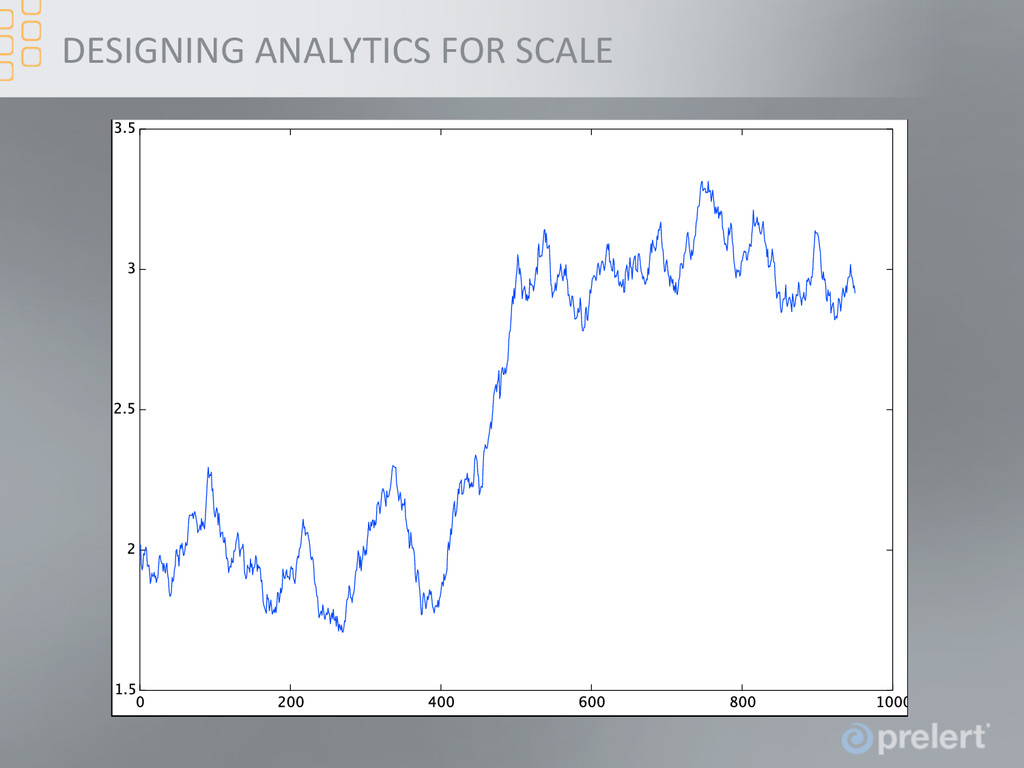
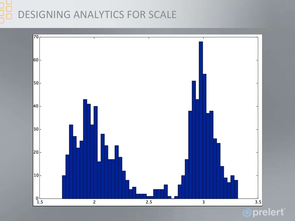
16. WHAT  YOU  MEASURE  IS  IMPORTANT  –  EXAMPLE   •  For  the  Fme  series  discussed  earlier  the  correlaFon  of   increments  between  adjacent  values  increased  at  the   Fme  of  the  change   •  For  example,  look  at  increments’  sliding  window   variance,  i.e.          and  the  change  is  clear  
17. WHAT  YOU  MEASURE  IS  IMPORTANT  –  EXAMPLE  
18. WHAT  YOU  MEASURE  IS  IMPORTANT  –  EXAMPLE  
19. DISTANCE  BASED  METHODS   •  Is  more  than  a  certain  fracFon,  f,  of  data  points  further   than  some  distance,  d,  from  the  point  (Knox,  Ng)   f  =  1   f  =  12/16  
20. DENSITY  BASED  METHODS   •  Local  outlier  factor,  compare  distance  from  the  point   to  its  neighbours          and  all  neighbours                          to  their   neighbours  (Breunig  et  al)   Not  outlier   Outlier  
21. PREDICTIVE  METHODS   •  When  a  dynamical  model  is  available  for  the  system,   i.e.  satellite,  plane,  etc.  Look  at  outliers  compared  to   the  predicFons  (residuals).  Kalman  filtering,   manoeuvre  detecFon,  etc   Outlier  
22. STATISTICAL   •  Robust  PCA     Low  rank   Sparse   Small  and  rank  full  
23. COMMONALITY   •  What  are  these  trying  to  do?   •  Es,mate  some  probability  density  func,on  and  then   look  for  points  in  the  tails  of  that  distribu,on   •  Distance  amounts  to  this  when  clusters  are  uniform   density,  and  this  is  the  case  where  it  works   •  Local  outlier  factor  tries  to  account  for  cluster  density   impact  on  distribuFon   •  PredicFve  model  amounts  to  path  dependent   probability  distribuFon   •  Robust  PCA  is  esFmaFng  the  probability  density   funcFon  when  it  lies  in  a  subspace  and  doing  it   robustly  
24. DENSITY  BASED  METHODS  –  REVISITED   •  Contour  lines  would  be  level  sets  of  a  probability   density  funcFon  that  would  be  a  reasonable  fit  to   these  points  
25. DENSITY  BASED  METHODS  –  REVISITED   •  Part  of  my  talk  at  SIAM*  workshop  concerned  how  to   measure  the  anomalousness  of  an  outcome  in  a   principled  way  given  a  probability  distribuFon       *  Society  for  Industrial  and  Applied  MathemaFcs  
26. IS  THIS  THE  ANSWER?  
27. CONCENTRATION  OF  MEASURE   •  A  brief  diversion:  survival  theory   •  Assume  uniform  IID  points  in  an  interval   •  Probability  that  the  nearest  neighbour  is  at  least       •  Assumes  r    is  small  compared  to  total  volume  
28. CONCENTRATION  OF  MEASURE   •  What  about  in  two  dimensions?   •  In  n-­‐dimensions  volume  of  shell  is     •  Points  become  increasingly  uniform   •  People  have  suggested  alternaFve  metrics  which  don’t   suffer  this  problem  to  the  same  extent  (see  for   example  Aggarwal  et  al)  
29. CONCENTRATION  OF  MEASURE  
30. CURSE  OF  DIMENSIONALITY   •  Previous  picture  a  bit  misleading   •  I  wasn’t  clear  about  the  constant  of  proporFonality.   Assumes  number  of  points  is  varying   •  Suppose  you  have  10  points  to  esFmate  density  in  1   dimension  (using  Kernel  Density  EsFmator)   •  Need  100  to  get  the  same  resoluFon  in  2  dimensions   •  In  general,  you  need                for  the  same  resoluFon   •  So  in  10  dimensions  you  need  10,000,000,000  points   •  InteresFngly,  the  same  problem  also  afflicts  models   with  more  parameters  
31. CURSE  OF  DIMENSIONALITY  –  SIMPLE  EXPERIMENT   •  Consider  the  case  of  esFmaFng  the  probability  of   seeing  more  extreme  sample  from  spherically   symmetric  mulFvariate  normal   •  EsFmate  sample  mean  and  full  covariance  matrix,  i.e.   D  +  D  (D  +  1)  /  2  parameters   •  Compute  probability  as  1-­‐F  (r  ),  where  F  (r  )  is  the   generalized  CDF  (see  here)   •  Fix  a  “3  sigma  point”,  red  crosses  in  figures.  (Note  that   r  of  point  with  constant  probability  varies  with   dimension)   •  EsFmate  using  100  samples  of  spherically  symmetric   mulFvariate  normal  and  repeat  500  Fmes  
32. CURSE  OF  DIMENSIONALITY  –  SIMPLE  EXPERIMENT   •  For  higher  dimensions  we  get  really  large  variaFon  in   the  magnitude  of  the  probability  up  to  106  across  our   500  trials   •  Can’t  just  esFmate  a  model  and  then  use  it  to   compute  probability  of  more  extreme  sample  without   understanding  variaFon  due  to  possible  errors  in   esFmaFng  model  parameters   •  Consider  bootstrap  or  Bayesian  approach  to   understand  uncertainty  in  assessment  of  how   anomalous  an  event  is  
33. CURSE  OF  DIMENSIONALITY  –  SIMPLE  EXPERIMENT  
34. CURSE  OF  DIMENSIONALITY  –  SIMPLE  EXPERIMENT  
35. CURSE  OF  DIMENSIONALITY  –  SIMPLE  EXPERIMENT  
36. IMPLICATIONS   •  In  high  dimensions   –  Data  are  very  uniform   –  Data  are  very  sparse   •  Advice:  full  mul,variate  analysis  is  not  effec,ve  for   anomaly  detec,on  in  high  dimensions   •  Can  be  possible  when  the  data  are  near  some  low   dimensional  manifold,  or  if  there  are  constraints  on   the  joint  distribuFon,  for  example  some  independence   •  You  need  a  principled  way  to  aggregate  measures  of   anomalousness  on  the  distribuFon  factors  
37. WARNING   •  Insight  is  not  always  equivalent  to  acFonability   •  Telling  a  system  administrator  that  his/her  system   “is  opera.ng  in  the  tails  of  its  distribu.on  about    the  low  dimensional  manifold  that  describes  its    typical  behaviour  on  a  Monday  morning”          is  likely  to  be  met  with  a  blank  expression   •  AcFonability  is  a  funcFon  of  user  experFse   •  Good  visualizaFons  always  help   •  Note  this  is  different  from  correlaFon  between   anomalies,  which  is  always  of  interest,  easy  to   understand,  and  useful  for  root  cause  analysis  
38. HOW  DO  YOU  DO  ANOMALY   DETECTION  IN  MACHINE  DATA?  
39. MACHINE  DATA  CHARACTERISTICS   •  Periodic  (daily  and  weekly)   •  Sporadic  features  (bank  holidays)   •  Domain  restricted  (percentages)   •  Heterogeneous  (error  messages,  codes,  counters,   performance  metrics,  IP  addresses  …)   •  CorrelaFons  (load  balancing)   •  Random  (non-­‐Gaussian  residuals,  more  later)   •  CharacterisFcs  constantly  evolving  (machines  brought   online,  new  users  arrive,  exisFng  users  leave)   •  Data  stream   •  Variable  data  rates  
40. MACHINE  DATA  IS  BIG  DATA   •  >1,000,000  performance  metrics  for  a  big  system   •  Thousands  of  events  per  second   •  People  are  indexing  mulFple  terabytes  of  data  a  day   and  NetFlow  data,  packet  header  informaFon,  is  much   bigger  
41. DESIGNING  ANALYTICS  FOR  SCALE   •  Map  reducible  features  allow  one  to  compress  the   data  near  where  its  stored  and  only  pass  the   compressed  data  to  the  anomaly  detecFon  processes,   provided  it  is  combinable   •  At  Prelert  we  use  aggregate  value  staFsFcs  like  count,   minimum,  maximum  and  mean  metric  values  in   short(ish)  Fme  intervals   •  More  complex  features,  such  as  least  squares   regression  coefficients,  can  also  be  computed  in  this   way  
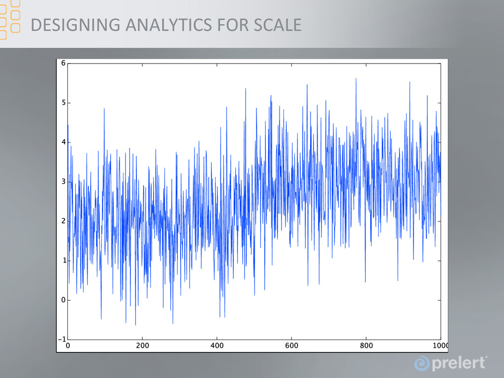
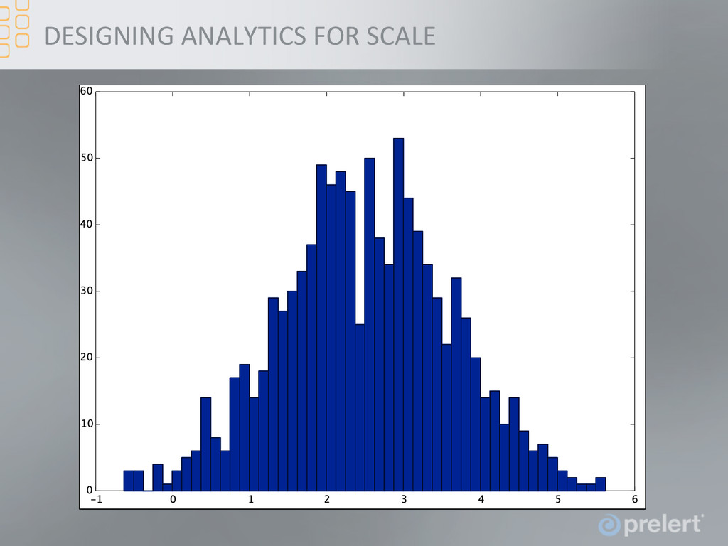
42. DESIGNING  ANALYTICS  FOR  SCALE   •  Allows  us  to  scale  and  means  the  runFme  of  the   analyFcs  are  predictable  at  very  different  data  rates   •  One  might  think  that  this  is  a  disadvantage  in  terms  of   accuracy.  However,  gives  different  insight  into  the   data  (for  simple  bulk  and  structure  anomaly  detecFon)   •  In  the  following  Fme  series,  the  process  mean   changes,  but  only  by  small  amount  compared  to  the   addiFve  noise   •  However,  the  change  is  clear  when  looking  at  the  Fme   window  means  
43. DESIGNING  ANALYTICS  FOR  SCALE  
44. DESIGNING  ANALYTICS  FOR  SCALE  
45. DESIGNING  ANALYTICS  FOR  SCALE  
46. DESIGNING  ANALYTICS  FOR  SCALE  
47. DESIGNING  ANALYTICS  FOR  SCALE   •  Online  algorithms  typically  get  to  see  each  piece  of   data  exactly  once   •  Suitable  for  data  streaming  environment,  parFcularly   where  data  characterisFcs  are  evolving   •  Also  allow  one  to  scale  to  arbitrarily  large  data  sets,   provided  one  can  keep  up  with  the  data  rate   •  OpFmizaFon  also  possible  when  the  objecFve  is   amenable,  i.e.  SGD  family  of  techniques   •  Can  make  things  challenging,  such  as  clustering   •  Advice:  it’s  worth  it  
48. ANALYTICS  CASE  STUDY  –  PERIODICITY   •  Periodicity  is  a  good  predictor  for  many  real  world  data   sets   •  Advice:  no  danger  of  over  fiRng  there’s  plenty  of  data   so  use  fully  non-­‐parametric  approach   •  InteresFngly,  if                                                          and                  is  mean  zero               •  Is  solved  by    
49. ANALYTICS  CASE  STUDY  –  PERIODICITY   •  Bucket  data,  compute  means  and  then  adapt  standard   spline  formulaFon  to  handle  mean  value  constraint   rather  than  knot  value  constraints  (very  efficient   eliminaFons  sFll  exist)   •  Splines  are  parFcularly  well  suited  to  cases  when  there   are  near  step  changes  or  periodic  spikes   •  Means  can  be  computed  online  storing  only  the  current   mean  and  count   •  Advice:  always  think  about  your  memory  QoR  curve,   i.e.  adapt  your  bucke,ng  so  that  it  has  its  highest   resolu,on  where  func,on  is  changing  fastest  
50. ANALYTICS  CASE  STUDY  –  CLUSTERING   •  Clustering  data  streams  is  hard  because  irreversible   decisions  can  have  bad  consequences   •  Advice:  avoid  making  them  if  at  all  possible   •  Sketch  data  structures  help  here,  see  for  example  BIRCH   •  If  you  are  using  mixture  models,  say  a  mixture  of   Gaussians,  think  about  the  memory  QoR  curve  again,  i.e.   using  spherically  symmetric  verses  full  covariance   matrices  means  that  you  can  use  more  components  for   the  same  total  memory  
51. ANALYTICS  CASE  STUDY  –  CLUSTERING  
52. ANALYTICS  CASE  STUDY  –  CLUSTERING  
53. ANALYTICS  CASE  STUDY  –  CLUSTERING  
54. ANALYTICS  CASE  STUDY:  TAIL  BEHAVIOUR   •  The  Normal  DistribuFon  doesn’t  visually  appear  to   be  too  bad.  However,  for  anomaly  detecFon  the  key   part  of  model  is  the  tail  of  the  distribuFon:   •  The  error  in  calculaFng  the  probability  of  values   becomes  more  and  more  significant  with  the  Normal   DistribuFon   •  Given  there  are  3263  samples  and  4  samples  are  >   12  Prelert’s  probability  (10e-­‐3)  is  a  more  reasonable   esFmate  than  the  Normal  distribuFon  (10e-­‐6)   Value Reference Probability* Probability Using Normal Distribution Probability Using Prelert 1 1 0.319498 0.560764 2 0.71835734 0.620394 0.834183 3 0.493717438 0.996086 0.49202 4 0.329757892 0.613486 0.27675 5 0.200122587 0.314752 0.157113 6 0.121973644 0.132196 0.0906333 7 0.065277352 0.0448887 0.0532552 8 0.033404842 0.0122142 0.0318895 9 0.033404842 0.00264629 0.0194524 10 0.015629789 0.000454401 0.012078 11 0.006435795 6.16E-05 0.00762581 12 0.002758198 6.58E-06 0.00489119 13 0.001225866 5.53E-07 0.00318382 14 0.000919399 3.65E-08 0.00210125 15 0.000612933 1.89E-09 0.00140482 16 ? 7.64E-11 0.000950655 17 ? 2.42E-12 0.000650663 18 ? 6.01E-14 0.000450111 19 ? 1.17E-15 0.000314514 20 ? 1.77E-17 0.000221852 * Tuned kernel estimate 1.00E+00   1.00E+01   1.00E+02   1.00E+03   1.00E+04   1.00E+05   1.00E+06   1   2   3   4   5   6   7   8   9   10   11   12   13   14   15   Error  Magnitude  (log  Scale)   Normal   DistribuFon   Anomalies  (<1%  probability)  
55. Thanks  
56. QuesFons?   tveasey@prelert.com