Structure of a shear-line polar low during a cold-air outbreak: comparing observations and Met Office Unified Model forecast

Transcript

1. Structure of a shear-line polar low during a cold-air outbreak: comparing observations and Met Office Unified Model forecast Denis Sergeev
2. Objectives  To investigate the structure of the shear-line polar low (PL)  To validate the model against airborne and remote-sensing observations Why is this case interesting?  One of less than a dozen of PLs and the first shear-line case ever observed with an instrumental aircraft  Representative for many mesoscale vortices forming in cold-air outbreaks near Svalbard
3. Outline: PL over the Norwegian Sea, 26 March 2013  Synoptic overview  Observational data  Numerical simulations (model set-up)  Results  Large-scale features  Cloud cover  Surface wind field  Mesoscale structure of the shear line  Wind and temperature fields  Cloud structure  Surface fluxes  Summary & challenges ahead
4. Synoptic perspective Data source: ERA-Interim reanalysis 6-hourly product  Stationary large-scale depression over the Norwegian Sea  Dominant throughout the period of the PL development  In the rear part: intense N cold-air outbreak (MCAO index > 7)  SST – T500 ≈ 50 K  Strong upper-level IPV anomaly Isentropic PV at 285K surface (shaded), SLP (red contours)
5. Synoptic perspective height (contours) and temperature (shaded) 850 hPa 500 hPa
7. Synoptic perspective: vertical wind field 00:00 UTC 700 hPa 10E longitude
8. Synoptic perspective: vertical wind field 06:00 UTC 700 hPa 10E longitude
9. Synoptic perspective: vertical wind field 12:00 UTC 700 hPa 10E longitude
10. Synoptic perspective: vertical wind field 18:00 UTC 700 hPa 10E longitude
11. The observed PL: some facts  Life cycle duration ≈ 1.5 days  Translation speed & direction ≈ 28.3 km/h, WNW  Total track length ≈1180 km  Diameter ~100-150 km  Cloud top height ~5-6 km  Environment:  ‘Mixed’ shear conditions  Weak conditional instability  Genesis:  Convergence of flow in the lee of Svalbard  Colliding vorticity filaments
12. Observational data In-situ: ACCACIA field campaign FAAM BAe-146 aircraft  Standard equipment [Renfrew et al., 2009]  Lidar, cloud water probes 11 dropsondes Remote: satellite data  Surface wind: ASCAT  Cloud cover: AVHRR  Cloud composition: CloudSat Photo by Rhiannon Davies
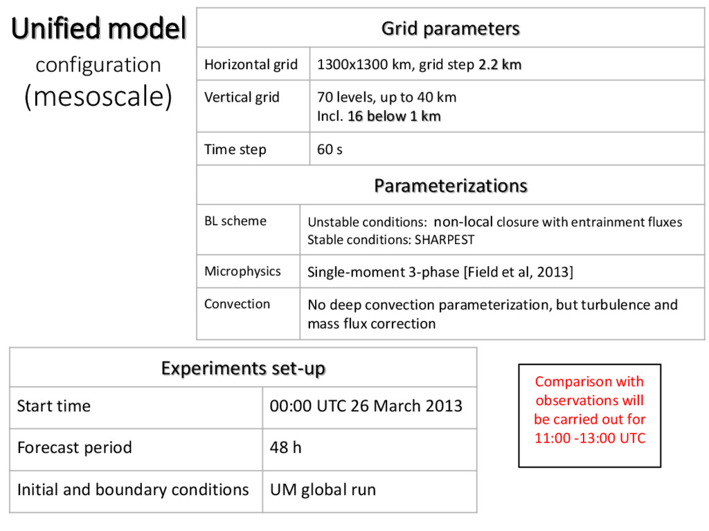
13. Unified model configuration (mesoscale) Grid parameters Horizontal grid 1300x1300 km, grid step 2.2 km Vertical grid 70 levels, up to 40 km Incl. 16 below 1 km Time step 60 s Parameterizations BL scheme Unstable conditions: non-local closure with entrainment fluxes Stable conditions: SHARPEST Microphysics Single-moment 3-phase [Field et al, 2013] Convection No deep convection parameterization, but turbulence and mass flux correction Experiments set-up Start time 00:00 UTC 26 March 2013 Forecast period 48 h Initial and boundary conditions UM global run Comparison with observations will be carried out for 11:00 -13:00 UTC
14. Observations vs UM: general picture Infra-red AVHRR image UM LW radiation at TOA SLP (red contours)
15. Observations vs UM: general picture ASCAT-A UM
16. Meteorological parameters  Wind components  Temperature field  Humidity and cloud water content  Surface fluxes Validation methods  Qualitative analysis of maps, vertical cross-sections  Time series along flight legs  Interpolating UM forecast data to observations coordinates  ‘Shifting’ model data in space in time to find best fit Mesoscale structure of the PL
17. Low-level aircraft legs and UM forecast Height: 0-1100 m Black/Blue: Obs. Red: UM
18. Vertical cross-sections Data from dropsonde soundings and UM  Temperature and wind field are captured well  The shear line / PL is displaced in the model by up to ≈50 km
19. Vertical cross-sections Data from dropsonde soundings and UM  Simulated potential temperature field is more uniform horizontally  Wind field – sharper in the model
24. What about clouds?
25. Cloud structure: aircraft observations vs UM Descending leg Black/Blue: Obs. Red: UM Magenta: UM averaged Summary:  Very good agreement in temperature and wind field  FWC – overestimated  LWC – underestimated  Similar results in latest UM studies
26. Cloud structure: CloudSat’s radar vs UM
27. Surface heat fluxes  Total surface heat flux ≈ 500 W/m2  SHF –overestimated, LHF - underestimated
28. Polar low structure  Well-defined shear line (≈25m/s over 50 km)  Wind speed maximum is collocated with convective cloud ‘wall’ (4-5 km)  Rolling-up vorticity banners produced a series of mesocyclones => barotropic instability?  One of the largest (and observed) PL was represented by cyclonic vorticity maximum with d≈150km  The eye-like centre is associated with uniformly high temperatures, calm and clear conditions Model validation  Large-scale features are represented very well by the model  Surface wind: waves are better resolved than in ASCAT data => +/- biases  Mesoscale wave propagation: displaced northward (or lagged by 1h) and sharper than in aircraft observations  Frozen water content is overestimated, liquid water- underestimated  Convective cells: good agreement with satellite data  Sensible heat flux is largely overestimated Summary
29. Modelling Earlier initialisation time Numerical simulations with higher resolution up to 500 m Sensitivity to orography and sea-ice mask Analysis Vorticity budget Potential vorticity diagnostics Energy budget (?) Future work Thank you! Questions?
30. EXTRA