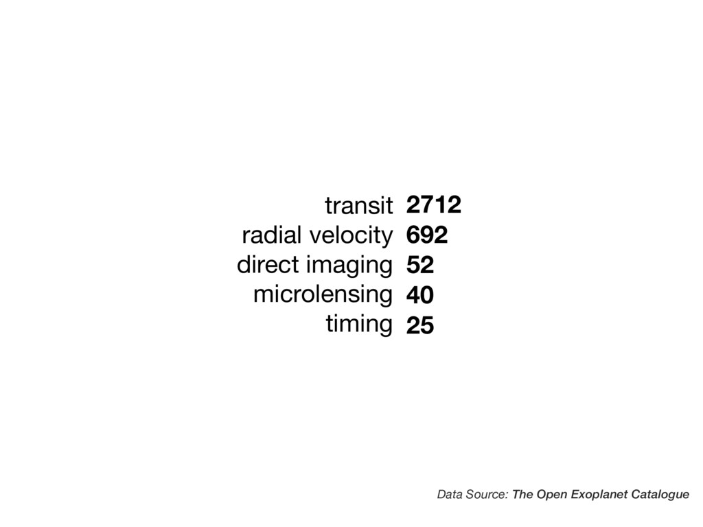
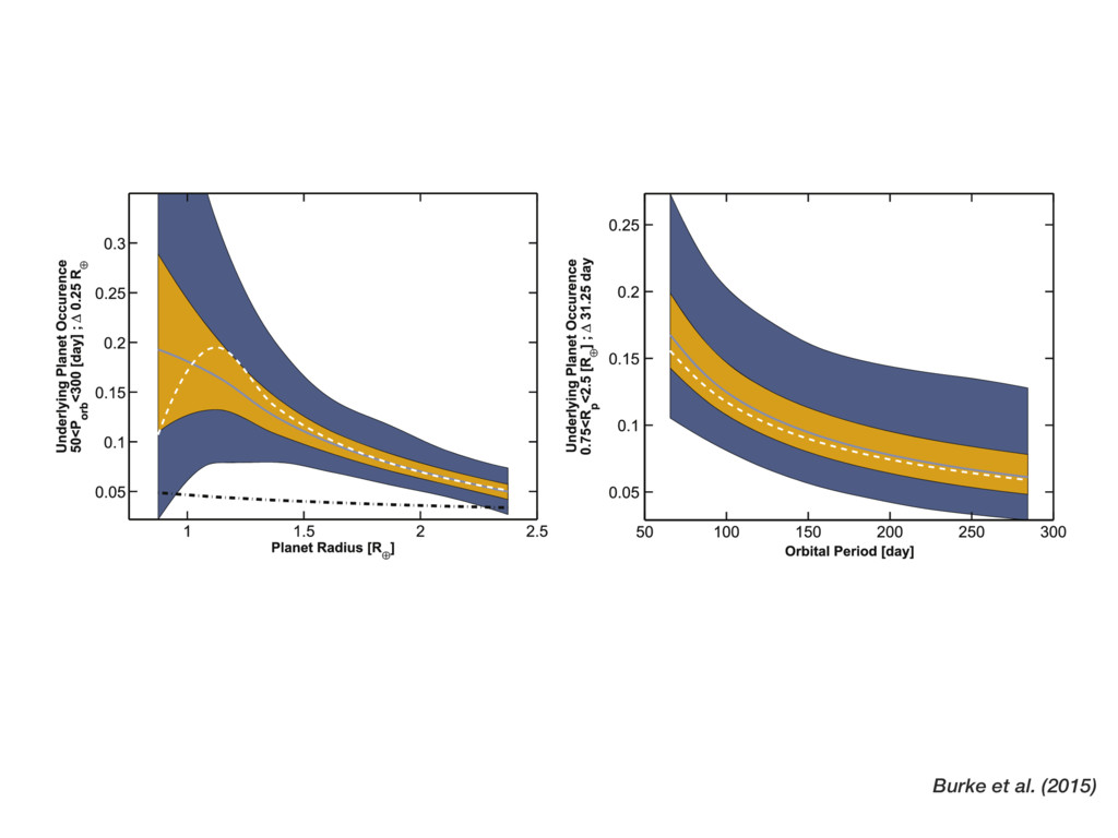
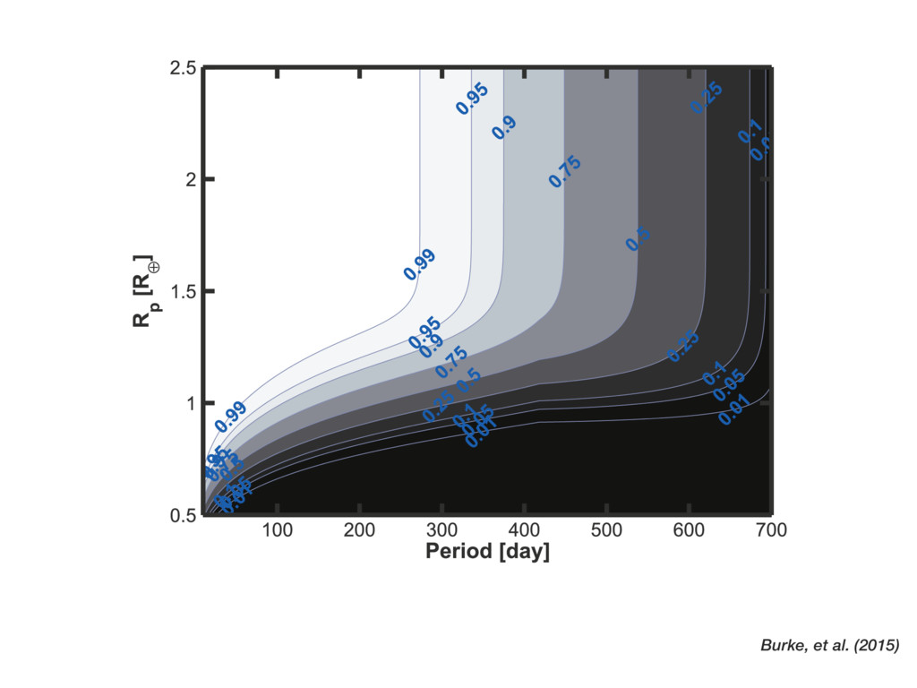
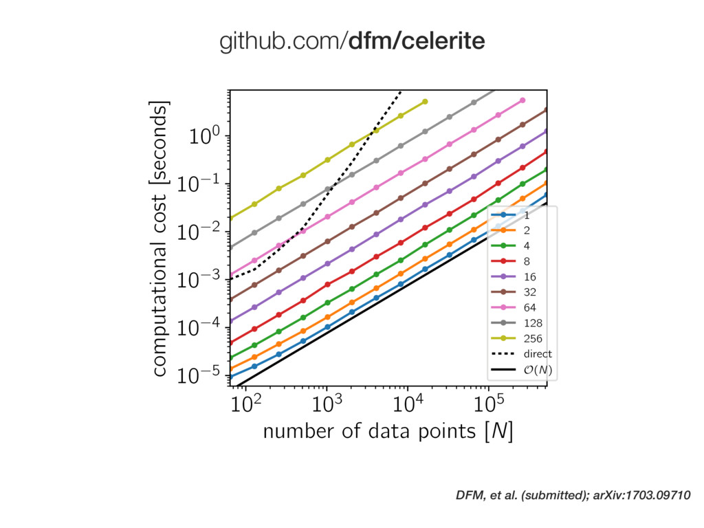
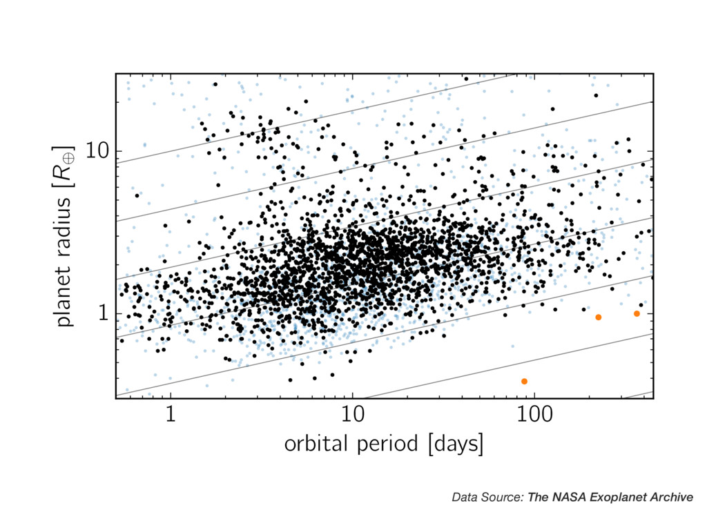
with a = -1.8 2 and has a break near the edge of the parameter space. Given the low numbers of observed planet candidates in the smallest planet bins, the full posterior allowed behavior (1σ orange region ; 3σ Figure 6) the occurrence rates in the smallest Rp bins. (b) The more complicated model ensures the ability to adapt to variations in the PLDF in the sensitivity analysis of Section 6.2. (c) Previous work on Kepler planet occurrence rates indicated a break in the planet population for 1 2.0 Rp 2.8 Å R (Fressin et al. 2013; Petigura et al. 2013a, 2013b; Silburt et al. 2015). (d) Finally, extending this work to a larger parameter space and for alternative target selection samples, such as the Kepler M dwarf sample where a sharp break at Rp ∼ 2.5 Å R is observed (Dressing & Charbonneau 2013; Burke et al. 2015), the double power law in Rp is strongly (BIC >10) warranted. Symptomatic of the weak evidence for a broken power law model over the ⩽ 0.75 Rp ⩽ 2.5 Å R range, Rbrk is not constrained within the prior Rp limits of the parameter space. When Rbrk is near the lower and upper Rp limits, a1 and a2 also become poorly constrained, respectively. To provide a more meaningful constraint on the average power law behavior for Rp in the double power law PLDF model, we introduce aavg , which we set to a a = avg 1 if ⩾ R R brk mid and a a = avg 2 otherwise, where Rmid is the midpoint between the upper and lower limits of Rp . We find a = -1.54 0.5 avg and b = -0.68 0.17 for our baseline result. We use aavg as a summary statistic for the model parameters only to enable a simpler comparison of our results to independent analyses of planet occurrence rates and to approximate the behavior for the power law Rp dependence if we had used the simpler single power law model. The results for a single power law model in both Rp and P orb are equivalent to the results for the double Figure 7. Same as Figure 6, but marginalized over 0.75 < Rp < 2.5 Å R and bins of dP orb = 31.25 days. Figure 8. Shows the underlying planet occurrence rate model. Marginalized over 50 < P orb < 300 days and bins of dRp =0.25 Å R planet occurrence rates for the model parameters that maximize the likelihood (white dash line). Posterior distribution for the underlying planet occurrence rate for the median (blue solid line), 1σ region (orange region), and 3σ region (blue region). An approximate PLDF based upon results from Petigura et al. (2013a) for comparison (dash dot line). Figure 9. Same as Figure 8, but marginalized over 0.75 < Rp < 2.5 Å R and bins of dP orb =31.25 days. Figure 6) the occurrence rates in the smallest Rp bins. (b) The more complicated model ensures the ability to adapt to variations in the PLDF in the sensitivity analysis of Section 6.2. (c) Previous work on Kepler planet occurrence rates indicated a break in the planet population for 1 2.0 Rp 2.8 Å R (Fressin et al. 2013; Petigura et al. 2013a, 2013b; Silburt et al. 2015). (d) Finally, extending this work to a larger parameter space and for alternative target selection samples, such as the Kepler M gure 7. Same as Figure 6, but marginalized over 0.75 < Rp < 2.5 Å R and bins dP orb = 31.25 days. Figure 9. Same as Figure 8, but marginalized over 0.75 < Rp < 2.5 Å R and bins of dP orb =31.25 days. he Astrophysical Journal, 809:8 (19pp), 2015 August 10 Burke et al.
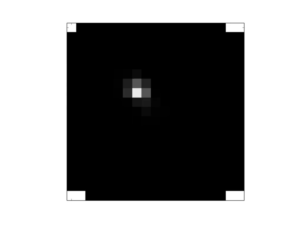
al. g by f the ough tudy, peline planet planet hlight matic with ng & e we e the ump- icity, Figure 1. Fractional completeness model for the host to Kepler-22b (KIC: 10593626) in the Q1-Q16 pipeline run using the analytic model described in Section 2. Burke et al.
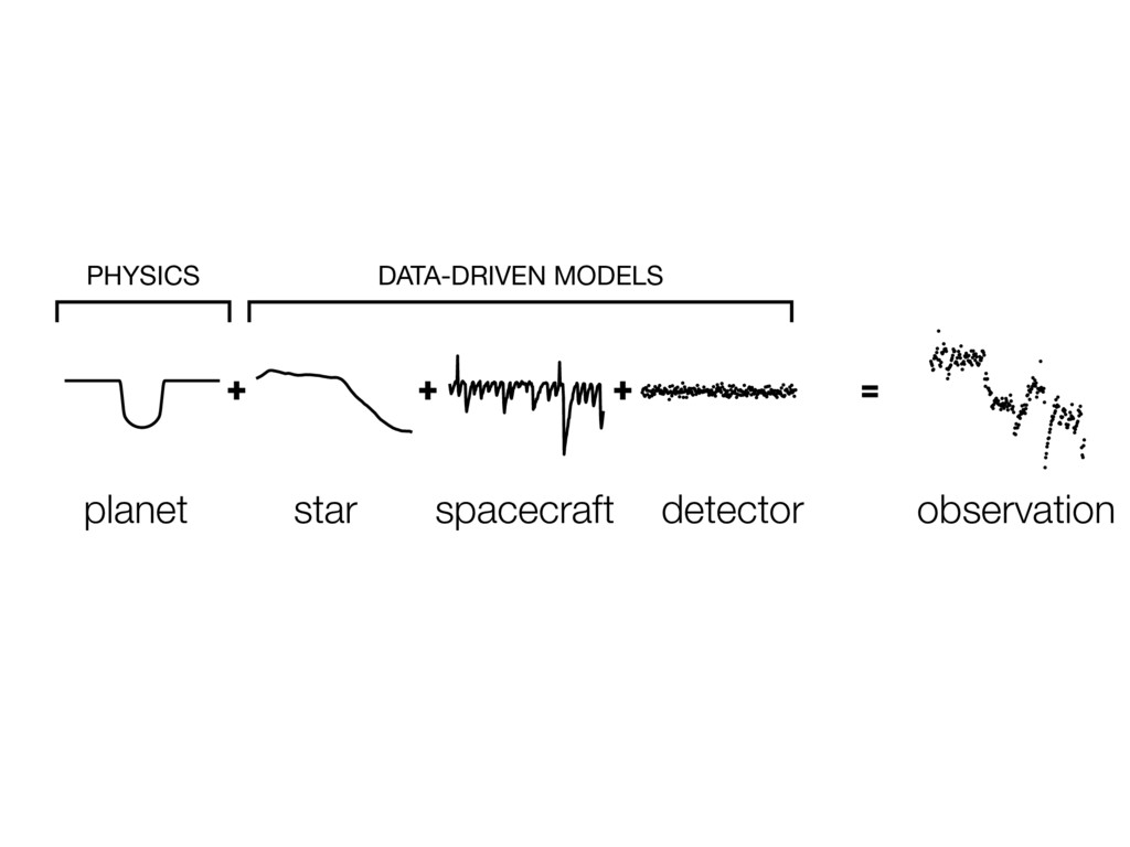
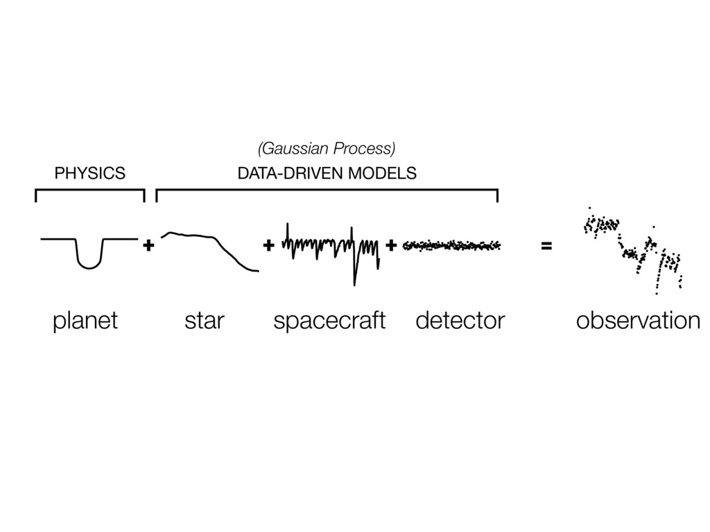
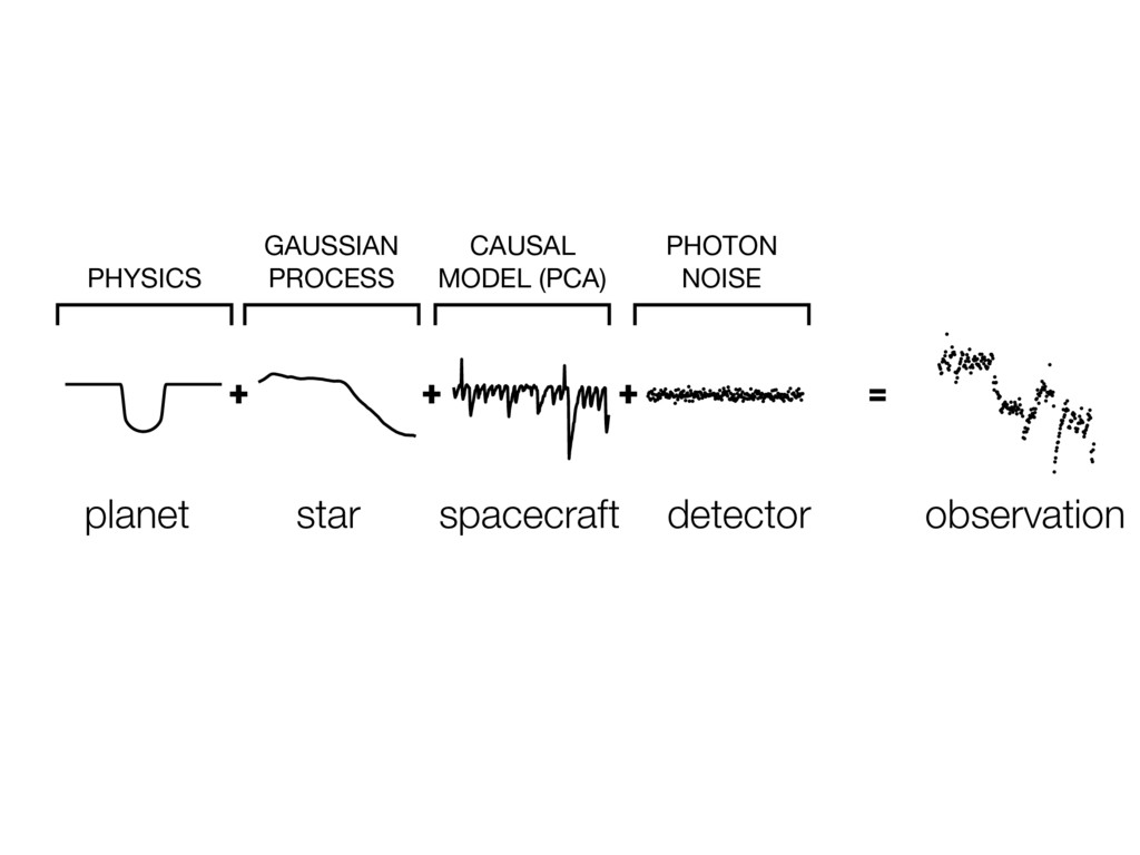
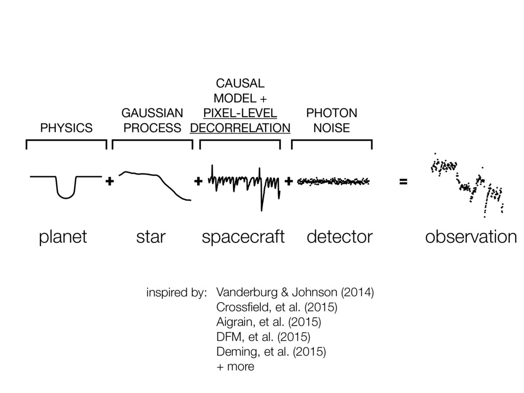
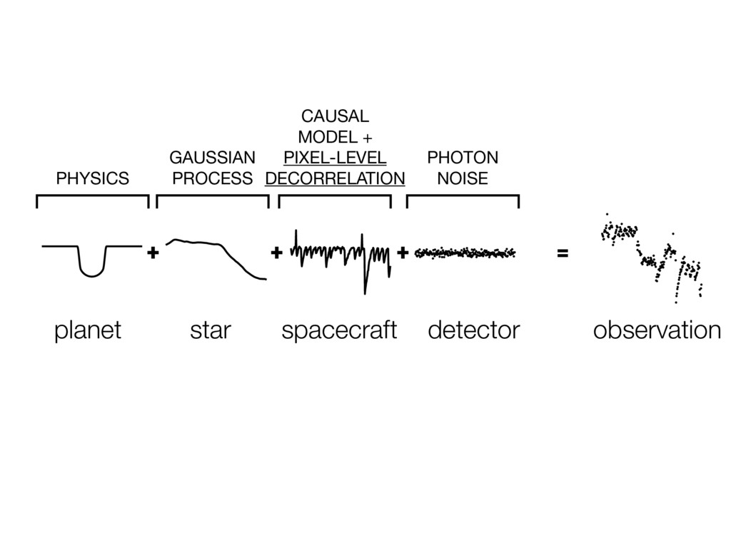
GAUSSIAN PROCESS CAUSAL MODEL + PIXEL-LEVEL DECORRELATION PHOTON NOISE inspired by: Vanderburg & Johnson (2014) Crossfield, et al. (2015) Aigrain, et al. (2015) DFM, et al. (2015) Deming, et al. (2015) + more
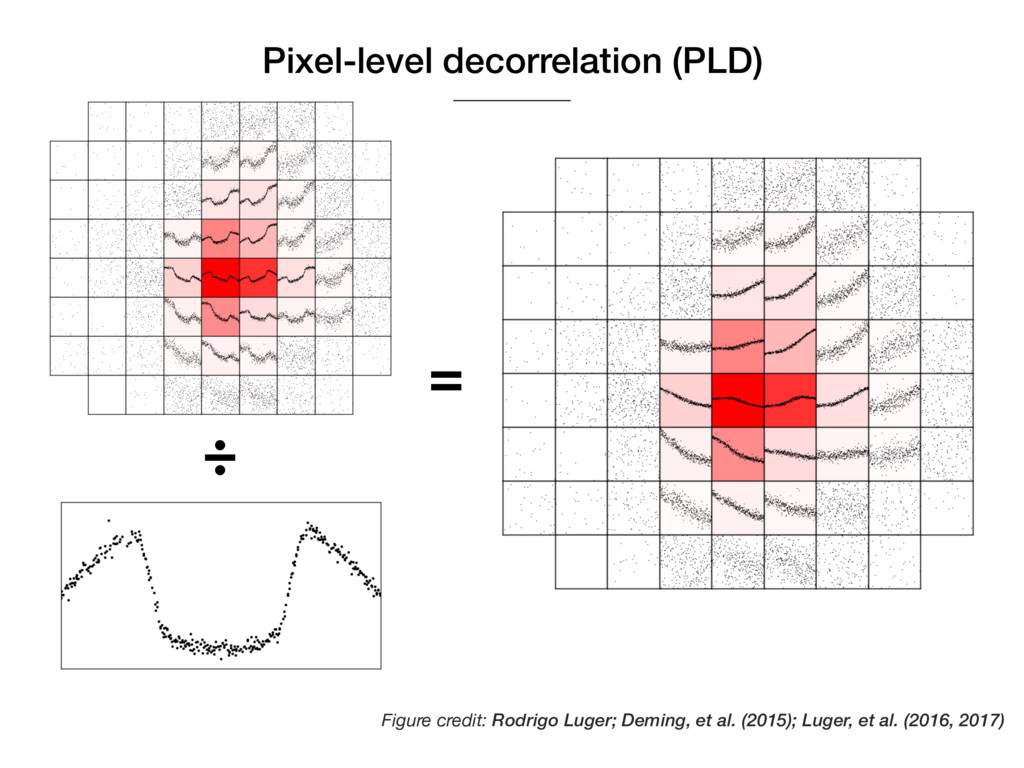
signal is multiplicative, then the fractional astrophysical contribution is equal in all pixels. Deming, et al. (2015); Luger, et al. (2016, 2017) ˆ pn(t) = pn(t) PN k=1 pn(t) estimator for instrumental signal estimator for astrophysical signal pixel time series
(WASP-47 e), a campaign 3 planet host. Show ter v in the validation set (red) and the scatter in the (blue) as a function of , the prior amplitude for Luger, Kruse, DFM, et al. (2017)
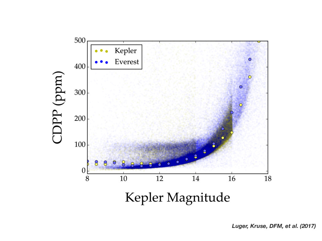
campaigns 3, 4, and 8, EVEREST recovers the Kepler precision dow of (variable) giant stars, leading to a higher average CDPP, while campaign 7 change in the orientation of the spacecraft and excess jitter. Fig. 20.— The same as Figure 19, but comparing the CDPP of all K2 stars to that of Kepler . EVEREST 2.0 recovers the original Kepler photometric precision down to at least Kp = 14, and past contam the in which inated valida fects o overfit spacec get ap of the apertu a time overfit § 3.7, o this be In F ing bin overfit light c binary
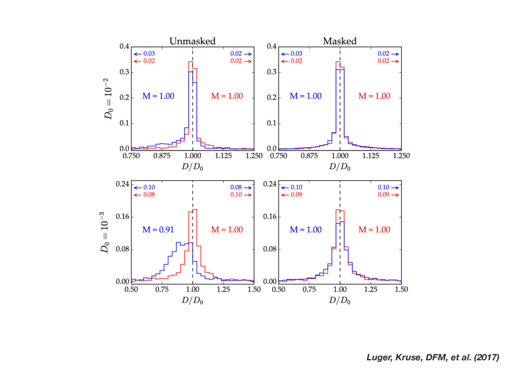
, and that e of the seg- 3, where we sections for e minimum al line indi- se between and slight re conserva- ith nPLD to report our and a com- arisons with curves. We proxy 6 hr h we calcu- we smooth clip outliers deviation in Luger, Kruse, DFM, et al. (2017)
90 100 110 0.985 0.990 0.995 1.000 1.005 −0.05 0.00 0.05 0.90 0.92 0.94 0.96 0.98 1.00 −0.06 −0.04 −0.02 0.00 0.02 0.04 0.06 −0.06 −0.04 −0.02 0.00 0.02 0.04 0.06 . . . . a b c d K2 long cadence data Barycentric Julian Date − 2,457,700 [day] Relative brightness Relative brightness 1b 1c 1d 1e 1f 1g 1h 1b 1c 1d 1e 1f 1g 1h Time from mid−transit [day] Relative brightness transit 1 transit 2 transit 3 transit 4 folded lightcurve Orbital separation [AU] Figure 1: a, b : Long cadence K2 light curve detrended with EVEREST and with stellar variability removed. Data points are in black, and our highest likelihood transit model for all seven planets TRAPPIST-1h: Luger, Sestovic, Kruse, et al. (2017); arXiv:1703.04166 embargoed
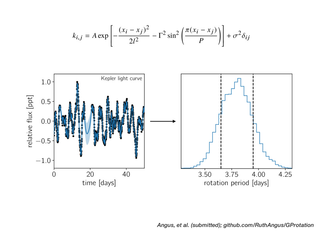
irements. We thus a method to prob- ation periods. This e rotation period, rtainty. arning community iology, geophysics used in the stellar e stellar variability l. 2012; Haywood 5; Haywood 2015; t al. 2015; Rajpaul eful in regression cifically when the variate Gaussian. If n in N dimensions, can describe that ocesses is provided tween data points demonstration, we ight curve of KIC s once every ⇠ 30.5 FGK stars. Clearly, summit of the Mauna Loa volcano in Hawaii (data from Keeling and Whorf 2004) using a kernel which is the product of a periodic and a SE kernel: the QP kernel. This kernel is defined as ki , j = A exp 2 6 6 6 6 4 ( xi xj )2 2 l 2 2 sin2 ⇡( xi xj ) P !3 7 7 7 7 5 + 2 ij . (2) It is the product of the SE kernel function, which describes the overall covariance decay, and an exponentiated, squared, sinusoidal kernel function that describes the periodic covariance structure. P can be interpreted as the rotation period of the star, and controls the amplitude of the sin2 term. If is very large, only points almost exactly one period away are tightly correlated and points that are slightly more or less than one period away are very loosely cor- related. If is small, points separated by one period are tightly correlated, and points separated by slightly more or less are still highly correlated, although less so. In other words, large values of lead to periodic variations with increasingly complex harmonic con- tent. This kernel function allows two data points that are separated in time by one rotation period to be tightly correlated, while also allowing points separated by half a period to be weakly correlated. The additional parameter captures white noise by adding a term to the diagonal of the covariance matrix. This can be interpreted to represent underestimation of observational uncertainties — if the uncertainties reported on the data are too small, it will be non- zero — or it can capture any remaining “jitter,” or residuals not captured by the e ective GP model. We use this QP kernel function (Equation 2) to produce the GP model that fits the Kepler light curve 0 20 40 time [days] 1.0 0.5 0.0 0.5 1.0 relative flux [ppt] Kepler light curve 10 1 100 ! [days 1] 10 3 10 2 10 1 S(!) power spectrum 0 0.000 0.025 0.050 0.075 0.100 0.125 k(⌧) 3.50 3.75 4.00 4.25 rotation period [days] Angus, et al. (submitted); github.com/RuthAngus/GProtation
![1.0 0.5 0.0 0.5 1.0 time since transit [days] 100](https://files.speakerdeck.com/presentations/61ed5b1f0cd848eeb761264f60ff7a7d/slide_21.jpg)
![1 10 100 orbital period [days] 1 10 planet radius](https://files.speakerdeck.com/presentations/61ed5b1f0cd848eeb761264f60ff7a7d/slide_62.jpg)
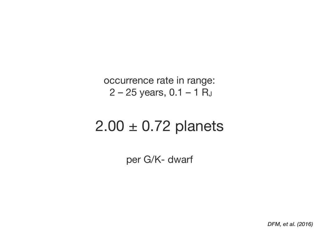
![DFM, et al. (2016) 3 5 10 20 period [years]](https://files.speakerdeck.com/presentations/61ed5b1f0cd848eeb761264f60ff7a7d/slide_77.jpg)
![1 10 100 1000 orbital period [days] 1 10 planet](https://files.speakerdeck.com/presentations/61ed5b1f0cd848eeb761264f60ff7a7d/slide_101.jpg)
![1 10 100 1000 orbital period [days] 1 10 planet](https://files.speakerdeck.com/presentations/61ed5b1f0cd848eeb761264f60ff7a7d/slide_102.jpg)