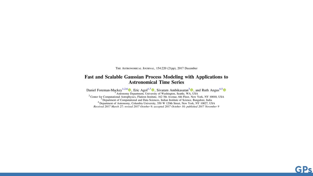
Astronomical Time Series Daniel Foreman-Mackey1,2,6 , Eric Agol1,7 , Sivaram Ambikasaran3 , and Ruth Angus4,5 1 Astronomy Department, University of Washington, Seattle, WA, USA 2 Center for Computational Astrophysics, Flatiron Institute, 162 5th Avenue, 6th Floor, New York, NY 10010, USA 3 Department of Computational and Data Sciences, Indian Institute of Science, Bangalore, India 4 Department of Astronomy, Columbia University, 550 W 120th Street, New York, NY 10027, USA Received 2017 March 27; revised 2017 October 9; accepted 2017 October 10; published 2017 November 9 Abstract The growing field of large-scale time domain astronomy requires methods for probabilistic data analysis that are computationally tractable, even with large data sets. Gaussian processes (GPs) are a popular class of models used for this purpose, but since the computational cost scales, in general, as the cube of the number of data points, their application has been limited to small data sets. In this paper, we present a novel method for GPs modeling in one dimension where the computational requirements scale linearly with the size of the data set. We demonstrate the method by applying it to simulated and real astronomical time series data sets. These demonstrations are examples of probabilistic inference of stellar rotation periods, asteroseismic oscillation spectra, and transiting planet parameters. The method exploits structure in the problem when the covariance function is expressed as a mixture of complex exponentials, without requiring evenly spaced observations or uniform noise. This form of covariance arises naturally when the process is a mixture of stochastically driven damped harmonic oscillators—providing a physical motivation for and interpretation of this choice—but we also demonstrate that it can be a useful effective The Astronomical Journal, 154:220 (21pp), 2017 December https://doi.org/10.3847/1538-3881/a © 2017. The American Astronomical Society. All rights reserved. Fast and Scalable Gaussian Process Modeling with Applications to Astronomical Time Series Daniel Foreman-Mackey1,2,6 , Eric Agol1,7 , Sivaram Ambikasaran3 , and Ruth Angus4,5 1 Astronomy Department, University of Washington, Seattle, WA, USA 2 Center for Computational Astrophysics, Flatiron Institute, 162 5th Avenue, 6th Floor, New York, NY 10010, USA 3 Department of Computational and Data Sciences, Indian Institute of Science, Bangalore, India 4 Department of Astronomy, Columbia University, 550 W 120th Street, New York, NY 10027, USA Received 2017 March 27; revised 2017 October 9; accepted 2017 October 10; published 2017 November 9 Abstract The growing field of large-scale time domain astronomy requires methods for probabilistic data analysis that are computationally tractable, even with large data sets. Gaussian processes (GPs) are a popular class of models used for this purpose, but since the computational cost scales, in general, as the cube of the number of data points, their application has been limited to small data sets. In this paper, we present a novel method for GPs modeling in one dimension where the computational requirements scale linearly with the size of the data set. We demonstrate the method by applying it to simulated and real astronomical time series data sets. These demonstrations are examples of probabilistic inference of stellar rotation periods, asteroseismic oscillation spectra, and transiting planet parameters. The method exploits structure in the problem when the covariance function is expressed as a mixture of complex exponentials, without requiring evenly spaced observations or uniform noise. This form of covariance arises naturally when the process is a mixture of stochastically driven damped harmonic oscillators—providing a physical motivation for and interpretation of this choice—but we also demonstrate that it can be a useful effective model in some other cases. We present a mathematical description of the method and compare it to existing scalable GP methods. The method is fast and interpretable, with a range of potential applications within astronomical data analysis and beyond. We provide well-tested and documented open-source implementations of The Astronomical Journal, 154:220 (21pp), 2017 December https://doi.org/10.3847/1538-3881/aa9332 © 2017. The American Astronomical Society. All rights reserved.
![time domain astronomy Measure [something] as a function of time.](https://files.speakerdeck.com/presentations/30ec1733ca4a474e92d425efb13dedf8/slide_10.jpg)
![time domain astronomy Measure [something] as a function of time.](https://files.speakerdeck.com/presentations/30ec1733ca4a474e92d425efb13dedf8/slide_11.jpg)
![data: NASA Exoplanet Archive 1 10 100 orbital period [days]](https://files.speakerdeck.com/presentations/30ec1733ca4a474e92d425efb13dedf8/slide_16.jpg)
![data: NASA Exoplanet Archive 1 10 100 orbital period [days]](https://files.speakerdeck.com/presentations/30ec1733ca4a474e92d425efb13dedf8/slide_19.jpg)
![1 10 100 orbital period [days] 1 10 planet radius](https://files.speakerdeck.com/presentations/30ec1733ca4a474e92d425efb13dedf8/slide_20.jpg)
![1 10 100 1000 10000 orbital period [days] 1 10](https://files.speakerdeck.com/presentations/30ec1733ca4a474e92d425efb13dedf8/slide_21.jpg)
![1.0 0.5 0.0 0.5 1.0 time since transit [days] 100](https://files.speakerdeck.com/presentations/30ec1733ca4a474e92d425efb13dedf8/slide_29.jpg)
![GPs 102 103 104 105 number of data points [N]](https://files.speakerdeck.com/presentations/30ec1733ca4a474e92d425efb13dedf8/slide_72.jpg)
![GPs 102 103 104 105 number of data points [N]](https://files.speakerdeck.com/presentations/30ec1733ca4a474e92d425efb13dedf8/slide_73.jpg)
![1 10 100 1000 10000 orbital period [days] 1 10](https://files.speakerdeck.com/presentations/30ec1733ca4a474e92d425efb13dedf8/slide_76.jpg)