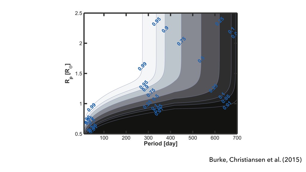
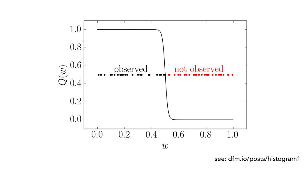
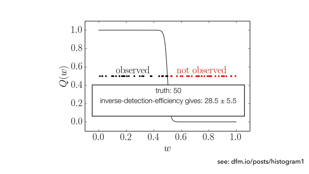
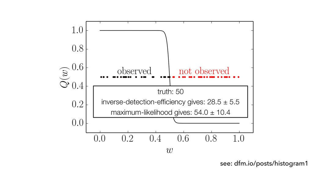
and igura et al. . hortcoming by eteness of the 2014) through s. In this study, Kepler pipeline rive the planet Kepler planet other highlight the systematic ce rates with ) and Dong & ysis where we recalculate the input assump- Figure 1. Fractional completeness model for the host to Kepler-22b (KIC: 10593626) in the Q1-Q16 pipeline run using the analytic model described in Section 2. t 10 Burke et al. Burke, Christiansen et al. (2015)
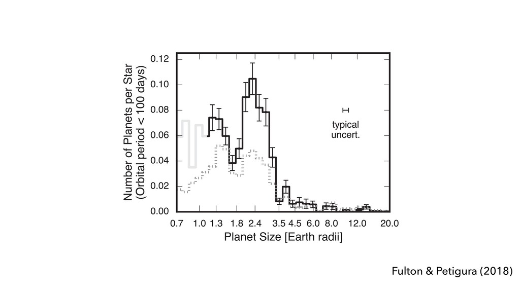
covariances w darkening duri After applying these Where possible, properties to the Ke radius and temper parameters. We cou stellar population b directed specificall population. After fil We calculated pla efficiency methodolo the detection sensit recovery tests perfo K02403.01 17.98 K00988.01 60.03 Note. This table contains filters described in Sectio (This table is available in Figure 5. The distribution of close-in planet sizes. The top panel shows the distribution from Fulton et al. (2017) and the bottom panel is the updated distribution from this work. The solid line shows the number of planets per star with orbital periods less than 100days as a function of planet size. A deep
covariances w darkening duri After applying these Where possible, properties to the Ke radius and temper parameters. We cou stellar population b directed specificall population. After fil We calculated pla efficiency methodolo the detection sensit recovery tests perfo K02403.01 17.98 K00988.01 60.03 Note. This table contains filters described in Sectio (This table is available in Figure 5. The distribution of close-in planet sizes. The top panel shows the distribution from Fulton et al. (2017) and the bottom panel is the updated distribution from this work. The solid line shows the number of planets per star with orbital periods less than 100days as a function of planet size. A deep
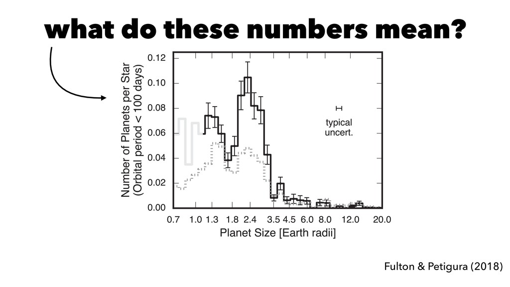
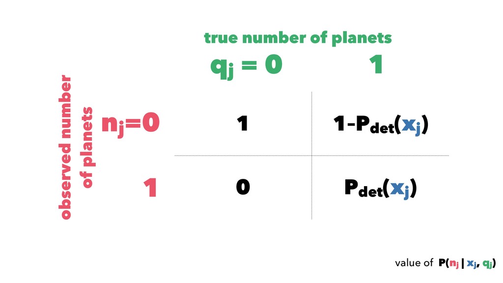
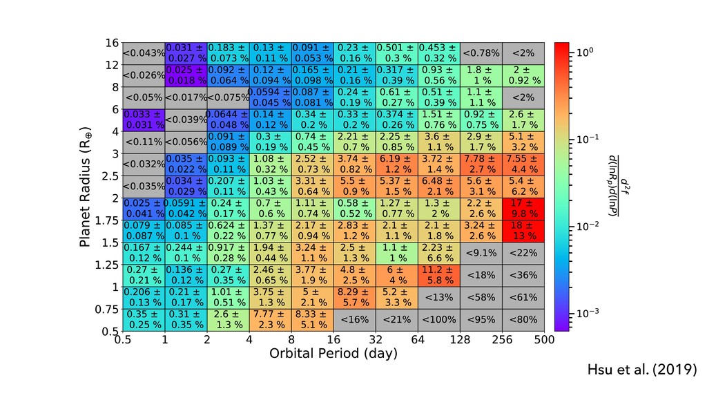
covariances w darkening duri After applying these Where possible, properties to the Ke radius and temper parameters. We cou stellar population b directed specificall population. After fil We calculated pla efficiency methodolo the detection sensit recovery tests perfo K02403.01 17.98 K00988.01 60.03 Note. This table contains filters described in Sectio (This table is available in Figure 5. The distribution of close-in planet sizes. The top panel shows the distribution from Fulton et al. (2017) and the bottom panel is the updated distribution from this work. The solid line shows the number of planets per star with orbital periods less than 100days as a function of planet size. A deep what do these numbers mean?
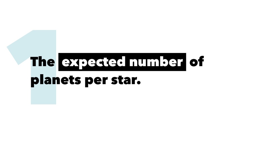
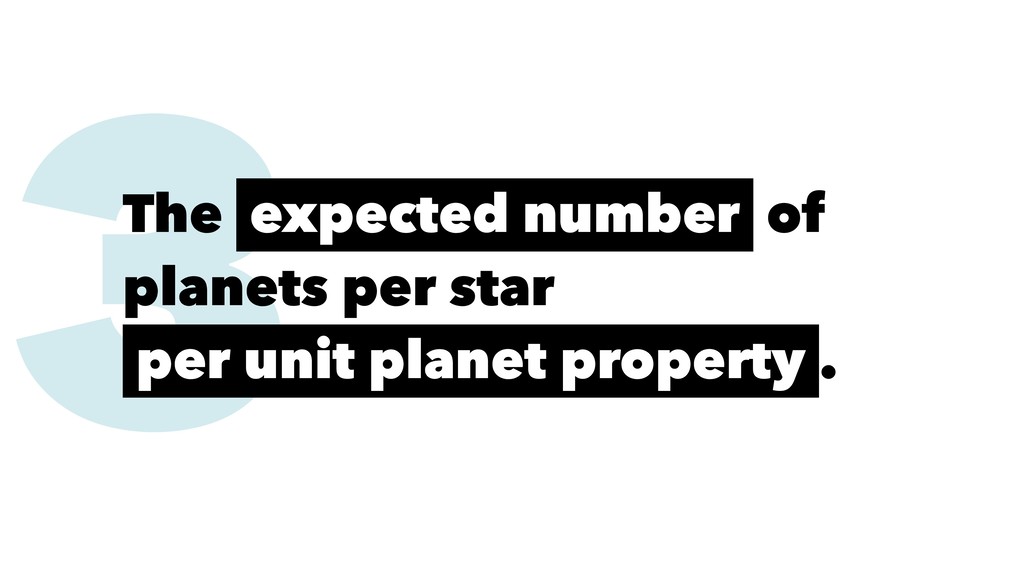
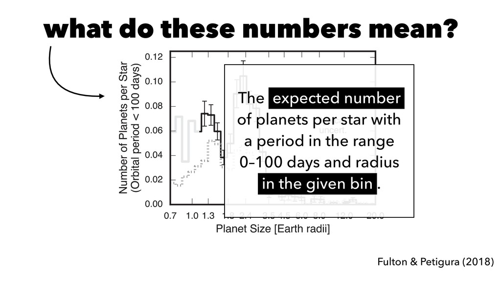
covariances w darkening duri After applying these Where possible, properties to the Ke radius and temper parameters. We cou stellar population b directed specificall population. After fil We calculated pla efficiency methodolo the detection sensit recovery tests perfo K02403.01 17.98 K00988.01 60.03 Note. This table contains filters described in Sectio (This table is available in Figure 5. The distribution of close-in planet sizes. The top panel shows the distribution from Fulton et al. (2017) and the bottom panel is the updated distribution from this work. The solid line shows the number of planets per star with orbital periods less than 100days as a function of planet size. A deep what do these numbers mean? The expected number of planets per star with a period in the range 0–100 days and radius in the given bin .
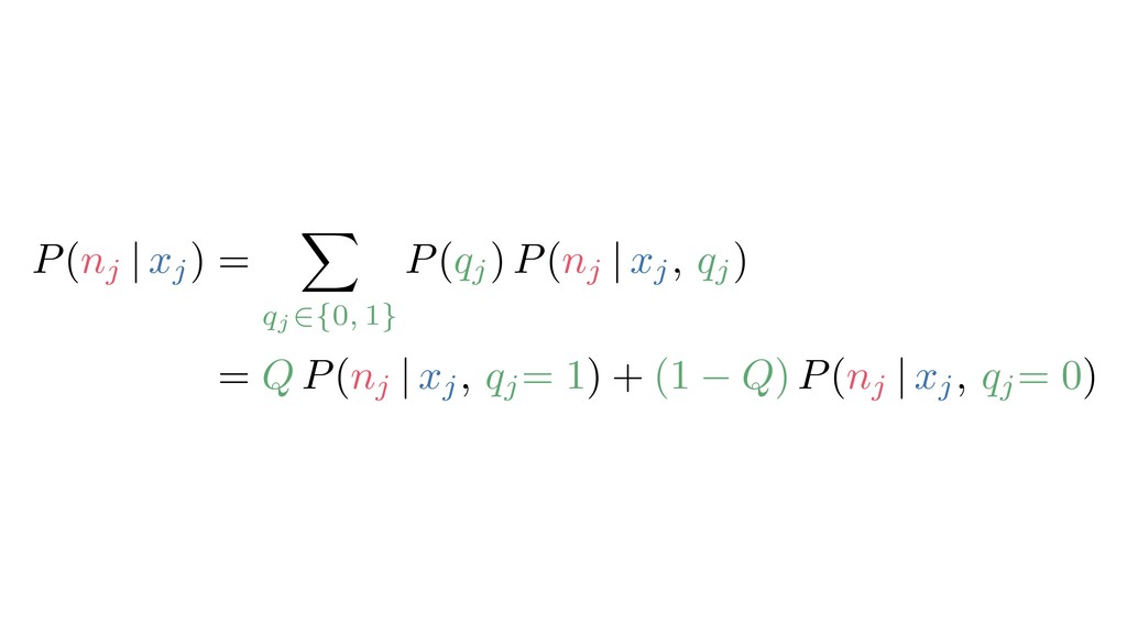
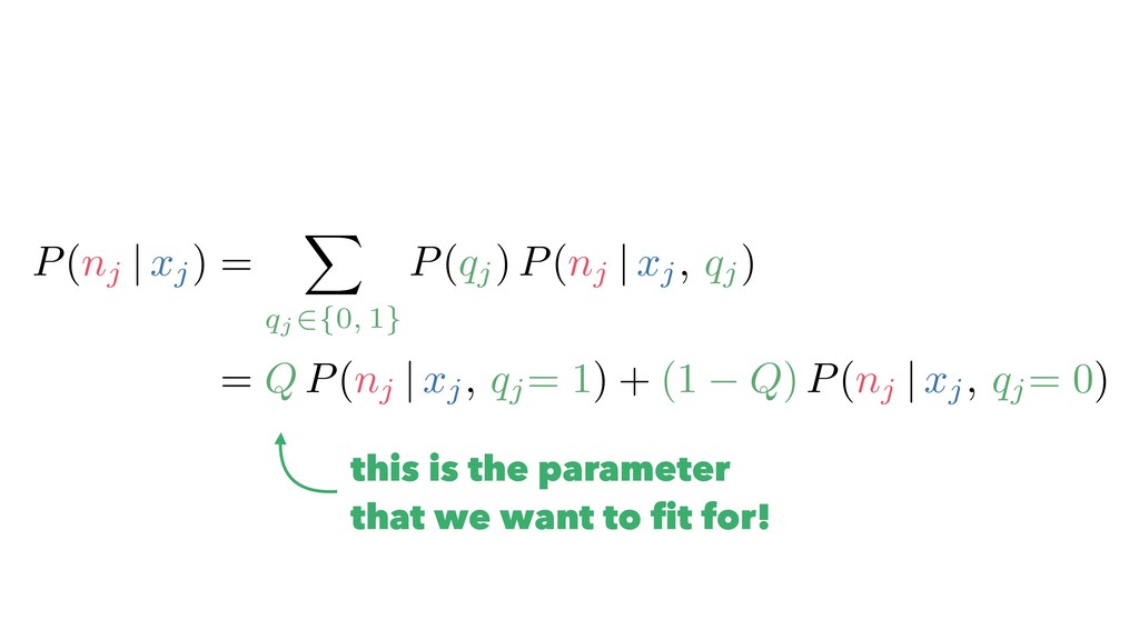
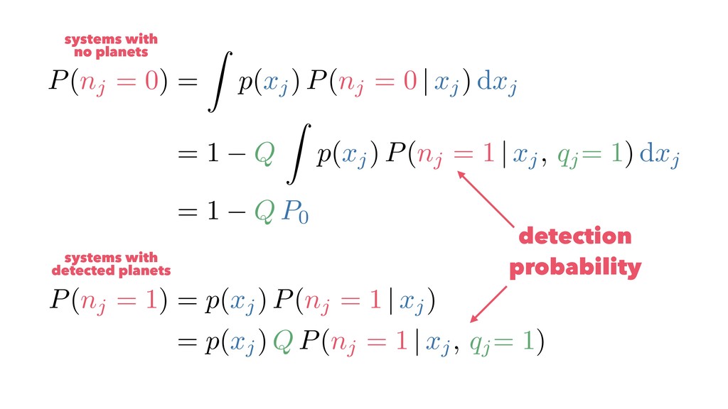
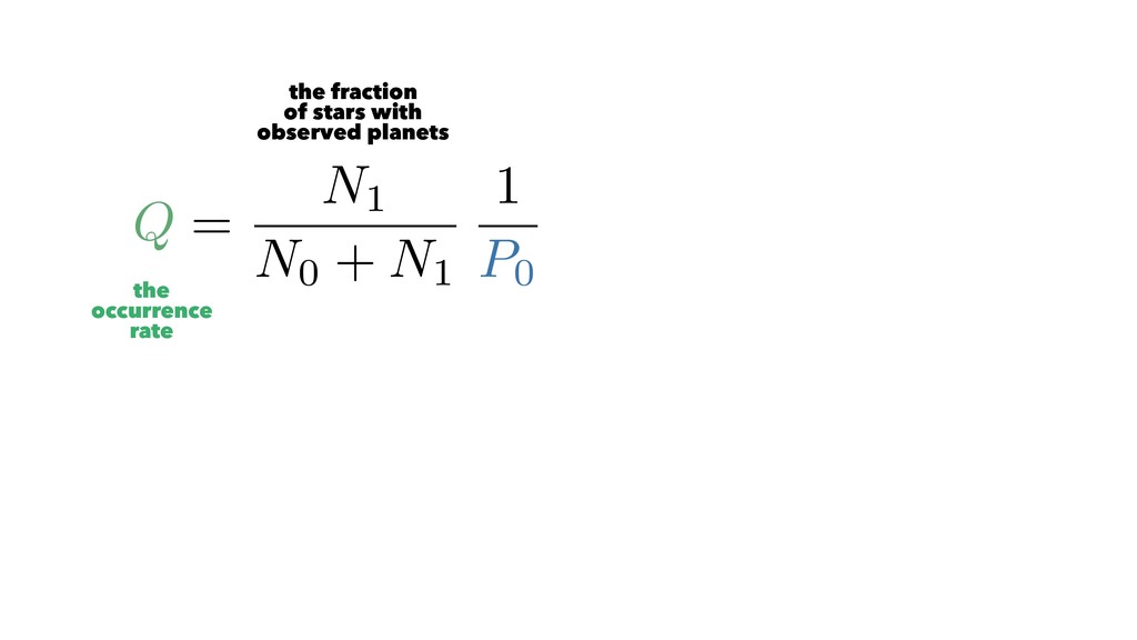
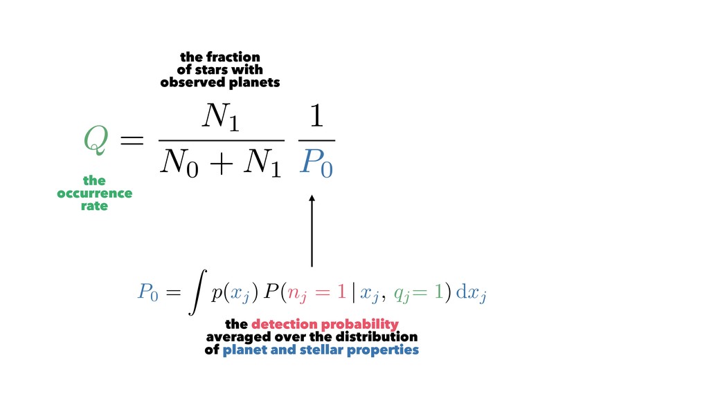
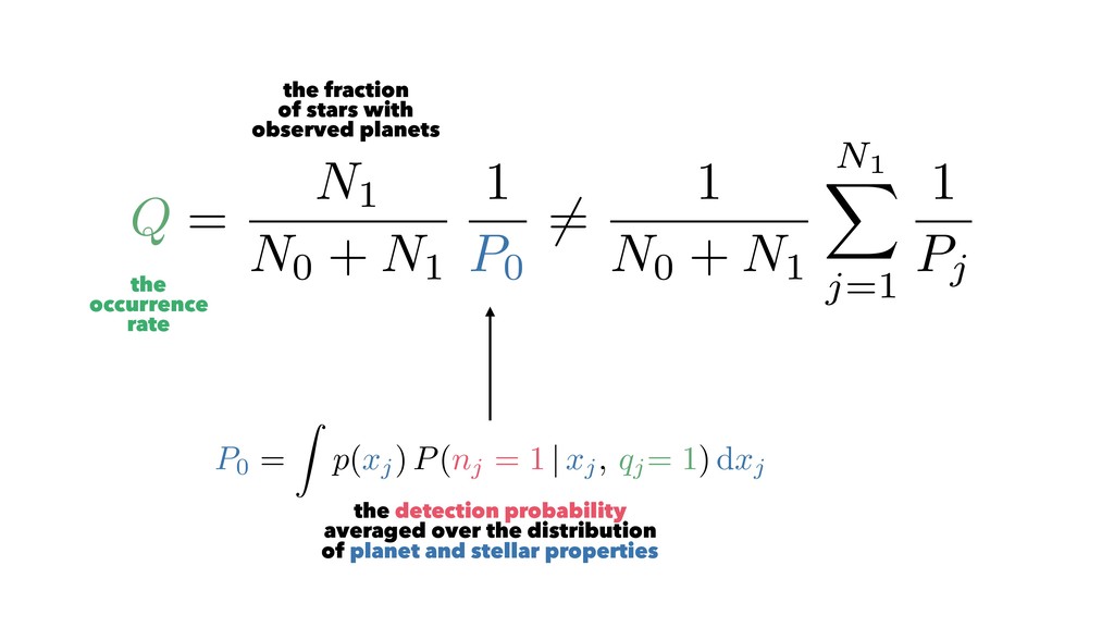
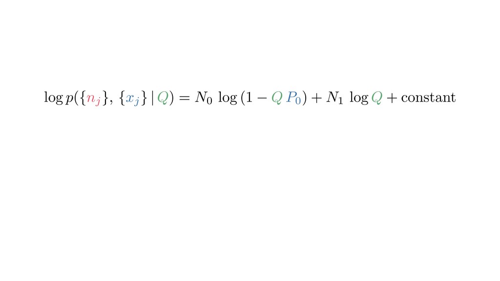
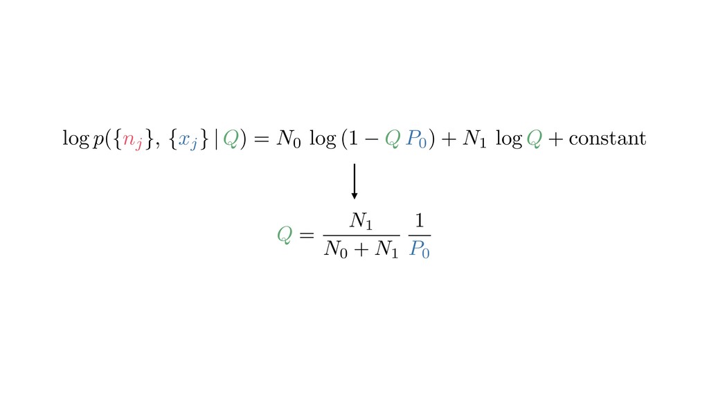
N0 + N1 N1 X j=1 1 Pj P0 = Z p(xj) P(nj = 1 | xj, qj= 1) dxj the detection probability averaged over the distribution of planet and stellar properties the occurrence rate the fraction of stars with observed planets
N0 + N1 N1 X j=1 1 Pj P0 = Z p(xj) P(nj = 1 | xj, qj= 1) dxj the detection probability averaged over the distribution of planet and stellar properties the occurrence rate the fraction of stars with observed planets
and igura et al. . hortcoming by eteness of the 2014) through s. In this study, Kepler pipeline rive the planet Kepler planet other highlight the systematic ce rates with ) and Dong & ysis where we recalculate the input assump- Figure 1. Fractional completeness model for the host to Kepler-22b (KIC: 10593626) in the Q1-Q16 pipeline run using the analytic model described in Section 2. t 10 Burke et al. Burke, Christiansen et al. (2015)
Kepler’s DR25 planet candidates associated with high-quality FGK target stars. These rares are based on a combined detection and vetting efficiency model that was fit to flux-level planet injection tests. The numerical values of the occurrence Hsu et al. (2019)
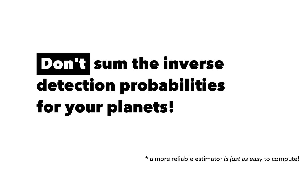
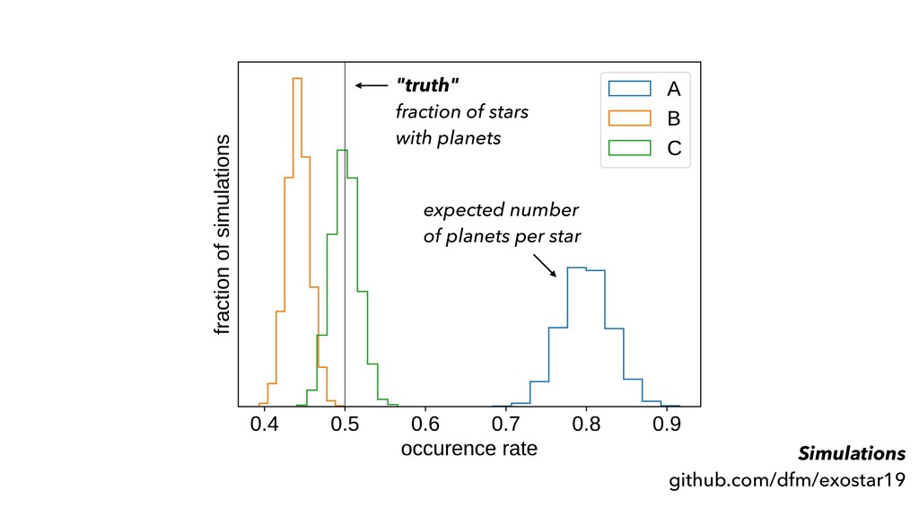
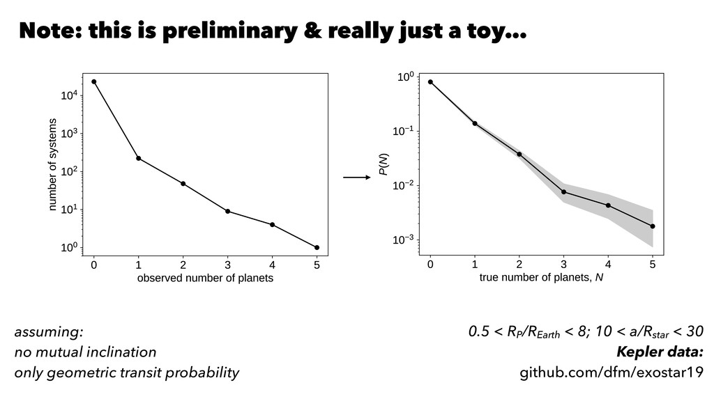
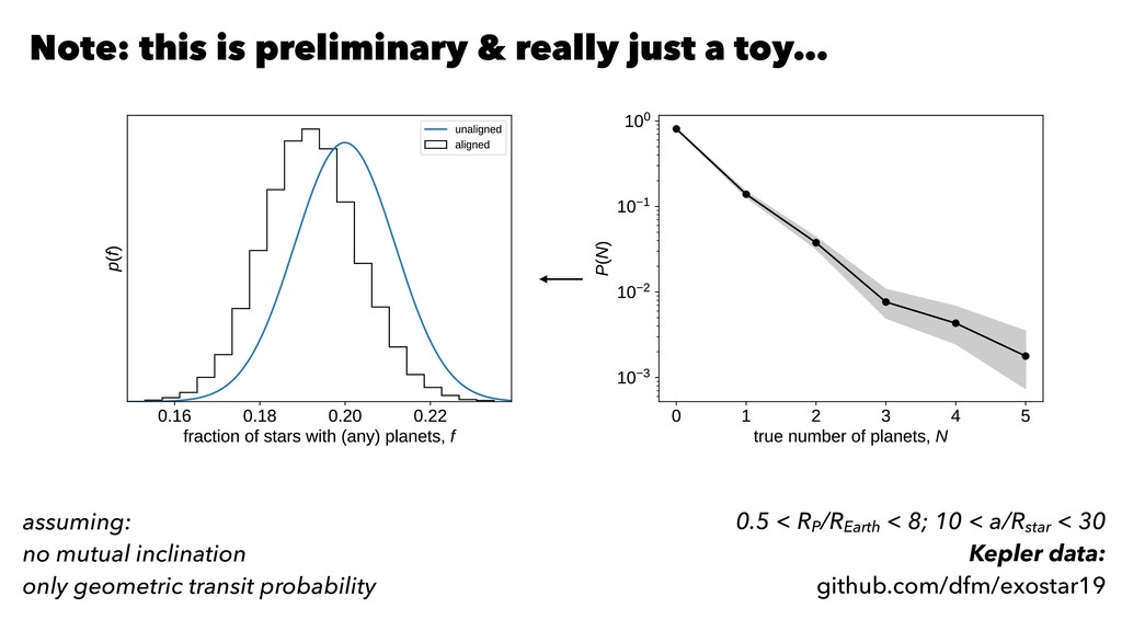
30 Kepler data: github.com/dfm/exostar19 Note: this is preliminary & really just a toy… assuming: no mutual inclination only geometric transit probability
![1 10 100 orbital period [days] 1 10 planet radius](https://files.speakerdeck.com/presentations/9d202d248a73424aa77f9a1f8a67f9f3/slide_3.jpg)
![1 10 100 orbital period [days] 1 10 planet radius](https://files.speakerdeck.com/presentations/9d202d248a73424aa77f9a1f8a67f9f3/slide_7.jpg)
![p({nj }, {xj } | Q) = [1 Q P0]N0](https://files.speakerdeck.com/presentations/9d202d248a73424aa77f9a1f8a67f9f3/slide_83.jpg)