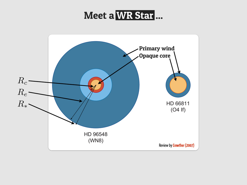
HD 66811 (O4 If) HD 164270 (WC9) Figure 5 Comparisons between stellar radii at Rosseland optical depths of 20 ( = R∗ , orange) and 2/3 ( = R2/3 , red ) for HD 66811 (O4 If ), HD 96548 (WR40, WN8), and HD 164270 (WR103, WC9), shown to scale. The primary optical wind line-forming region, 1011 ≤ ne ≤ 1012 cm−3, is shown in dark blue, plus higher density wind material, ne ≥ 1012 cm−3, is indicated in light blue. The figure illustrates the highly extended winds of ownloaded from www.annualreviews.org ARY on 02/28/12. For personal use only. 20 R(Sun) HD 96548 (WN8) HD 66811 (O4 If) HD 164270 (WC9) Figure 5 Comparisons between stellar radii at Rosseland optical depths of 20 ( = R∗ , orange) and 2/3 ( = R2/3 , red ) for HD 66811 (O4 If ), HD 96548 (WR40, WN8), and HD 164270 (WR103, WC9), shown to scale. The primary optical wind line-forming region, 1011 ≤ ne ≤ 1012 cm−3, is shown in dark blue, plus higher density wind material, ne ≥ 1012 cm−3, is indicated in light blue. The figure illustrates the highly extended winds of WR stars with respect to Of supergiants (Repolust, Puls & Herrero 2004; Herald, Hillier & Schulte-Ladbeck 2001; Crowther, Morris & Smith 2006b). evolutionary models, namely Primary wind Review by Crowther (2007) Opaque core Rc Re R⇤