Upgrade to Pro — share decks privately, control downloads, hide ads and more …

Introduction to IPython & Jupyter Notebooks

Introduction to IPython & Jupyter Notebooks

Introduction to IPython & Jupyter Notebooks
http://eueung.github.io/python/ipython-intro/

Eueung Mulyana

November 15, 2015
Tweet

More Decks by Eueung Mulyana

Other Decks in Technology

Transcript

  1. Agenda 1. Introduction to IPython 2. IPython QtConsole 3. Jupyter

    Notebook 4. Notebook: Getting Started 2 / 34
  2. One of Python’s most useful features is its interactive interpreter.

    It allows for very fast testing of ideas without the overhead of creating test files as is typical in most programming languages. However, the interpreter supplied with the standard Python distribution is somewhat limited for extended interactive use. IPython A comprehensive environment for interactive and exploratory computing Three Main Components: An enhanced interactive Python shell. A decoupled two-process communication model, which allows for multiple clients to connect to a computation kernel, most notably the web-based notebook. An architecture for interactive parallel computing. Some of the many useful features of IPython includes: Command history, which can be browsed with the up and down arrows on the keyboard. Tab auto-completion. In-line editing of code. Object introspection, and automatic extract of documentation strings from python objects like classes and functions. Good interaction with operating system shell. Support for multiple parallel back-end processes, that can run on computing clusters or cloud services like Amazon EC2. 4 / 34
  3. IPython provides a rich architecture for interactive computing with: A

    powerful interactive shell. A kernel for Jupyter. Easy to use, high performance tools for parallel computing. Support for interactive data visualization and use of GUI toolkits. Flexible, embeddable interpreters to load into your own projects. IPython IPython is an interactive shell that addresses the limitation of the standard python interpreter, and it is a work-horse for scientific use of python. It provides an interactive prompt to the python interpreter with a greatly improved user-friendliness. It comes with a browser-based notebook with support for code, text, mathematical expressions, inline plots and other rich media. You don’t need to know anything beyond Python to start using IPython – just type commands as you would at the standard Python prompt. But IPython can do much more than the standard prompt... 5 / 34
  4. IPython Beyond the Terminal ... The REPL as a Network

    Protocol Kernels Execute Code Clients Read input Present Output Simple abstractions enable rich, sophisticated clients 6 / 34
  5. The Four Most Helpful Commands The four most helpful commands

    is shown to you in a banner, every time you start IPython: Command Description ? Introduction and overview of IPython’s features. % q u i c k r e f Quick reference. h e l p Python’s own help system. o b j e c t ? Details about o b j e c t , use o b j e c t ? ? for extra details. Tab Completion Tab completion, especially for attributes, is a convenient way to explore the structure of any object you’re dealing with. Simply type o b j e c t _ n a m e . < T A B > to view the object’s attributes. Besides Python objects and keywords, tab completion also works on file and directory names. Running and Editing The % r u n magic command allows you to run any python script and load all of its data directly into the interactive namespace. Since the file is re-read from disk each time, changes you make to it are reflected immediately (unlike imported modules, which have to be specifically reloaded). IPython also includes d r e l o a d , a recursive reload function. % r u n has special flags for timing the execution of your scripts (- t ), or for running them under the control of either Python’s pdb debugger (- d ) or profiler (- p ). The % e d i t command gives a reasonable approximation of multiline editing, by invoking your favorite editor on the spot. IPython will execute the code you type in there as if it were typed interactively. 7 / 34
  6. Magic Functions ... The following examples show how to call

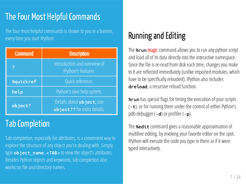
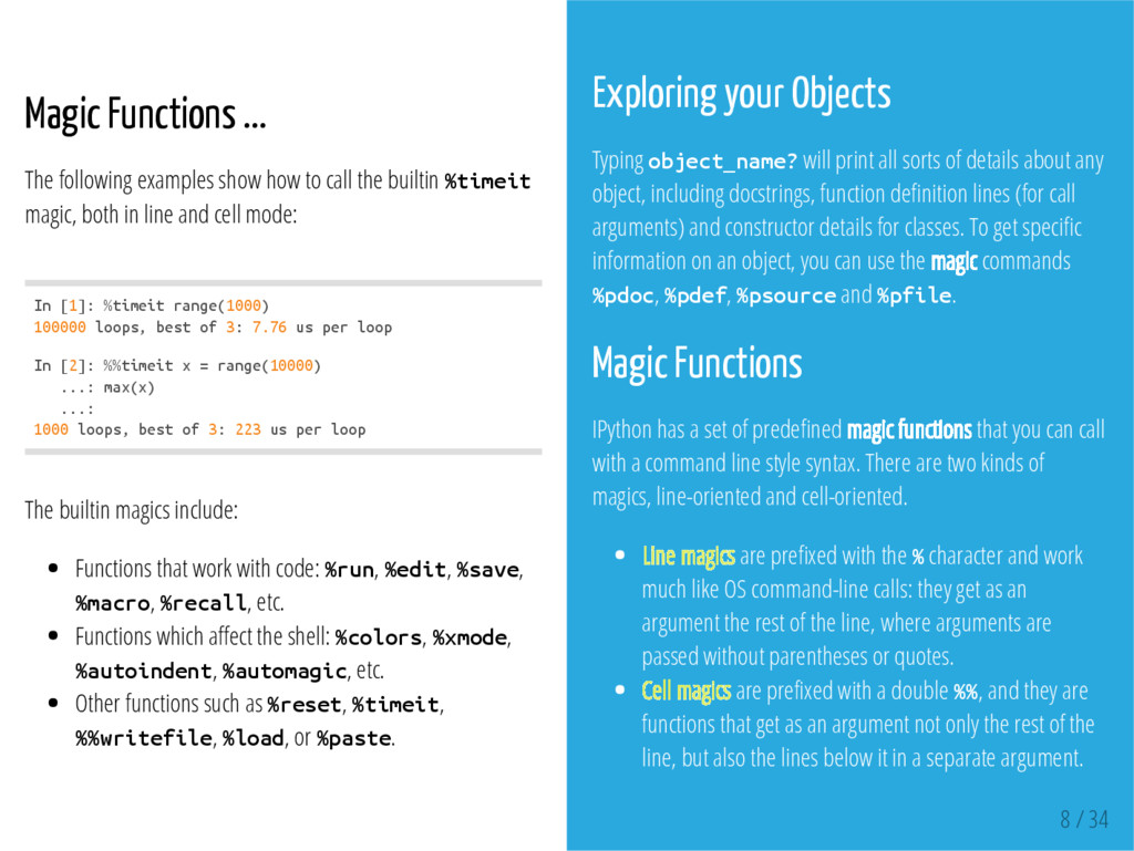
    the builtin % t i m e i t magic, both in line and cell mode: I n [ 1 ] : % t i m e i t r a n g e ( 1 0 0 0 ) 1 0 0 0 0 0 l o o p s , b e s t o f 3 : 7 . 7 6 u s p e r l o o p I n [ 2 ] : % % t i m e i t x = r a n g e ( 1 0 0 0 0 ) . . . : m a x ( x ) . . . : 1 0 0 0 l o o p s , b e s t o f 3 : 2 2 3 u s p e r l o o p The builtin magics include: Functions that work with code: % r u n , % e d i t , % s a v e , % m a c r o , % r e c a l l , etc. Functions which affect the shell: % c o l o r s , % x m o d e , % a u t o i n d e n t , % a u t o m a g i c , etc. Other functions such as % r e s e t , % t i m e i t , % % w r i t e f i l e , % l o a d , or % p a s t e . Exploring your Objects Typing o b j e c t _ n a m e ? will print all sorts of details about any object, including docstrings, function definition lines (for call arguments) and constructor details for classes. To get specific information on an object, you can use the magic commands % p d o c , % p d e f , % p s o u r c e and % p f i l e . Magic Functions IPython has a set of predefined magic functions that you can call with a command line style syntax. There are two kinds of magics, line-oriented and cell-oriented. Line magics are prefixed with the % character and work much like OS command-line calls: they get as an argument the rest of the line, where arguments are passed without parentheses or quotes. Cell magics are prefixed with a double % % , and they are functions that get as an argument not only the rest of the line, but also the lines below it in a separate argument. 8 / 34
  7. System Shell Commands To run any command at the system

    shell, simply prefix it with ! . You can capture the output into a Python list. To pass the values of Python variables or expressions to system commands, prefix them with $ . System Aliases It’s convenient to have aliases to the system commands you use most often. This allows you to work seamlessly from inside IPython with the same commands you are used to in your system shell. IPython comes with some pre-defined aliases and a complete system for changing directories, both via a stack (% p u s h d , % p o p d and % d h i s t ) and via direct %cd. The latter keeps a history of visited directories and allows you to go to any previously visited one. Magic Functions ... You can always call them using the % prefix, and if you’re calling a line magic on a line by itself, you can omit even that: r u n t h e s c r i p t . p y . You can toggle this behavior by running the % a u t o m a g i c magic. Cell magics must always have the % % prefix. A more detailed explanation of the magic system can be obtained by calling % m a g i c , and for more details on any magic function, call % s o m e m a g i c ? to read its docstring. To see all the available magic functions, call % l s m a g i c . System Shell Commands ... ! p i n g w w w . b b c . c o . u k f i l e s = ! l s # c a p t u r e ! g r e p - r F $ p a t t e r n i p y t h o n / * # p a s s i n g v a r s 9 / 34
  8. History ... Input and output history are kept in variables

    called In and Out, keyed by the prompt numbers. The last three objects in output history are also kept in variables named _ , _ _ and _ _ _ . You can use the % h i s t o r y magic function to examine past input and output. Input history from previous sessions is saved in a database, and IPython can be configured to save output history. Several other magic functions can use your input history, including % e d i t , % r e r u n , % r e c a l l , % m a c r o , % s a v e and % p a s t e b i n . You can use a standard format to refer to lines: % p a s t e b i n 3 1 8 - 2 0 ~ 1 / 1 - 5 This will take line 3 and lines 18 to 20 from the current session, and lines 1-5 from the previous session. History IPython stores both the commands you enter, and the results it produces. You can easily go through previous commands with the up- and down-arrow keys, or access your history in more sophisticated ways. Debugging After an exception occurs, you can call % d e b u g to jump into the Python debugger (pdb) and examine the problem. Alternatively, if you call % p d b , IPython will automatically start the debugger on any uncaught exception. You can print variables, see code, execute statements and even walk up and down the call stack to track down the true source of the problem. This can be an efficient way to develop and debug code, in many cases eliminating the need for print statements or external debugging tools. You can also step through a program from the beginning by calling % r u n - d t h e p r o g r a m . p y . 10 / 34
  9. To force multiline input, hit C t r l -

    E n t e r at the end of the first line instead of E n t e r S h i f t - E n t e r to execute! IPython QtConsole a version of IPython, using the new two-process ZeroMQ Kernel, running in a PyQt GUI a very lightweight widget that largely feels like a terminal, but provides a number of enhancements only possible in a GUI, such as inline figures, proper multiline editing with syntax highlighting, graphical calltips, and much more. # T o s t a r t t h e Q t C o n s o l e i p y t h o n q t c o n s o l e # T o s e e a q u i c k i n t r o d u c t i o n o f t h e m a i n f e a t u r e s % g u i r e f See: Qt Console @ RTD 12 / 34
  10. IPython QtConsole MF % l o a d The new

    % l o a d magic takes any script, and pastes its contents as your next input, so you can edit it before executing. The script may be on your machine, but you can also specify an history range, or a url, and it will download the script from the web. This is particularly useful for playing with examples from documentation, such as matplotlib. I n [ 6 ] : % l o a d h t t p : / / m a t p l o t l i b . o r g / p l o t _ d i r e c t i v e / m p l _ e x a m p l e I n [ 7 ] : f r o m m p l _ t o o l k i t s . m p l o t 3 d i m p o r t a x e s 3 d . . . : i m p o r t m a t p l o t l i b . p y p l o t a s p l t . . . : . . . : f i g = p l t . f i g u r e ( ) . . . : a x = f i g . a d d _ s u b p l o t ( 1 1 1 , p r o j e c t i o n = ' 3 d ' ) . . . : X , Y , Z = a x e s 3 d . g e t _ t e s t _ d a t a ( 0 . 0 5 ) . . . : c s e t = a x . c o n t o u r ( X , Y , Z ) . . . : a x . c l a b e l ( c s e t , f o n t s i z e = 9 , i n l i n e = 1 ) . . . : . . . : p l t . s h o w ( ) 13 / 34
  11. MF % l o a d ... The % l

    o a d magic can also load source code from objects in the user or global namespace by invoking the - n option. I n [ 1 ] : i m p o r t h e l l o _ w o r l d . . . : % l o a d - n h e l l o _ w o r l d . s a y _ h e l l o I n [ 3 ] : d e f s a y _ h e l l o ( ) : . . . : p r i n t ( " H e l l o W o r l d ! " ) Inline Matplotlib One of the most exciting features of the QtConsole is embedded matplotlib figures. You can use any standard matplotlib GUI backend to draw the figures, and since there is now a two- process model, there is no longer a conflict between user input and the drawing eventloop. 14 / 34
  12. If you have a reference to a matplotlib figure object,

    you can always display that specific figure: I n [ 1 ] : f = p l t . f i g u r e ( ) I n [ 2 ] : p l t . p l o t ( n p . r a n d ( 1 0 0 ) ) O u t [ 2 ] : [ < m a t p l o t l i b . l i n e s . L i n e 2 D a t 0 x 7 f c 6 a c 0 3 d d 9 0 > ] I n [ 3 ] : d i s p l a y ( f ) # P l o t i s s h o w n h e r e I n [ 4 ] : p l t . t i t l e ( ' A t i t l e ' ) O u t [ 4 ] : < m a t p l o t l i b . t e x t . T e x t a t 0 x 7 f c 6 a c 0 2 3 4 5 0 > I n [ 5 ] : d i s p l a y ( f ) # U p d a t e d p l o t w i t h t i t l e i s s h o w n h e r e . Matplotlib: d i s p l a y ( ) IPython provides a function d i s p l a y ( ) for displaying rich representations of objects if they are available. The IPython display system provides a mechanism for specifying PNG or SVG (and more) representations of objects for GUI frontends. When you enable matplotlib integration via the %matplotlib magic, IPython registers convenient PNG and SVG renderers for matplotlib figures, so you can embed them in your document by calling display() on one or more of them. This is especially useful for saving your work. I n [ 4 ] : f r o m I P y t h o n . d i s p l a y i m p o r t d i s p l a y I n [ 5 ] : p l t . p l o t ( r a n g e ( 5 ) ) # p l o t s i n t h e m a t p l o t l i b w i n d o w I n [ 6 ] : d i s p l a y ( p l t . g c f ( ) ) # e m b e d s t h e c u r r e n t f i g u r e i n t h e I n [ 7 ] : d i s p l a y ( * g e t f i g s ( ) ) # e m b e d s a l l a c t i v e f i g u r e s i n t h e 15 / 34
  13. - - m a t p l o t l

    i b i n l i n e If you want to have all of your figures embedded in your session, instead of calling d i s p l a y ( ) , you can specify - - m a t p l o t l i b i n l i n e when you start the console, and each time you make a plot, it will show up in your document, as if you had called d i s p l a y ( f i g ) ( ) . The inline backend can use either SVG or PNG figures (PNG being the default). To switch between them, set the InlineBackend.figure_format configurable in a config file, or via the % c o n f i g magic: I n [ 1 0 ] : % c o n f i g I n l i n e B a c k e n d . f i g u r e _ f o r m a t = ' s v g ' Changing the inline figure format also affects calls to display() above, even if you are not using the inline backend for all figures. I n [ 1 3 ] : [ f i g . c l o s e ( ) f o r f i g i n g e t f i g s ( ) ] By default, IPython closes all figures at the completion of each execution. It also means that the first matplotlib call in each cell will always create a new figure. However, it does prevent the list of active figures surviving from one input cell to the next, so if you want to continue working with a figure, you must hold on to a reference to it. I n [ 1 1 ] : p l t . p l o t ( r a n g e ( 1 0 0 ) ) < s i n g l e - l i n e p l o t > I n [ 1 2 ] : p l t . p l o t ( [ 1 , 3 , 2 ] ) < a n o t h e r s i n g l e - l i n e p l o t > # - - - - - I n [ 1 1 ] : f i g = g c f ( ) . . . . : f i g . p l o t ( r a n d ( 1 0 0 ) ) < p l o t > I n [ 1 2 ] : f i g . t i t l e ( ' R a n d o m T i t l e ' ) < r e d r a w p l o t w i t h t i t l e > This behavior is controlled by the InlineBackend.close_figures configurable, and if you set it to False, via %config or config file, then IPython will not close figures, and tools like gcf(), gca(), getfigs() will behave the same as they do with other backends. You will, however, have to manually close figures: 16 / 34
  14. Jupyter Notebook The Jupyter Notebook is a web application for

    interactive data science and scientific computing. Using the Jupyter Notebook, you can author engaging documents that combine live-code with narrative text, equations, images, video, and visualizations. By encoding a complete and reproducible record of a computation, the documents can be shared with others on GitHub, Dropbox, and the Jupyter Notebook Viewer. # I n s t a l l s u d o a p t - g e t i n s t a l l b u i l d - e s s e n t i a l p y t h o n - d e v p i p i n s t a l l j u p y t e r # S t a r t j u p y t e r n o t e b o o k # P r e v i o u s l y p i p i n s t a l l " i p y t h o n [ n o t e b o o k ] " i p y t h o n n o t e b o o k See: Jupyter@RTD 18 / 34
  15. Open source, interactive data science and scientific computing across over

    40 programming languages. The Jupyter Notebook is a web application that allows you to create and share documents that contain live code, equations, visualizations and explanatory text. Uses include: data cleaning and transformation, numerical simulation, statistical modeling, machine learning and much more. Language of Choice The Notebook has support for over 40 programming languages, including those popular in Data Science such as Python, R, Julia and Scala. Share Notebooks Notebooks can be shared with others using email, Dropbox, GitHub and the Jupyter Notebook Viewer. Interactive Widgets Code can produce rich output such as images, videos, LaTeX, and JavaScript. Interactive widgets can be used to manipulate and visualize data in realtime. Big-Data Integration Leverage big data tools, such as Apache Spark, from Python, R and Scala. Explore that same data with pandas, scikit-learn, ggplot2, dplyr, etc. See: Jupyter.ORG Website 19 / 34
  16. Project Jupyter The IPython Notebook (2011) Rich Web Client Text

    & Math Code Results Share, Reproduce. See: Fernando Perez, IPython & Project Jupyter 20 / 34
  17. Project Jupyter IPython Interactive Python shell at the terminal Kernel

    for this protocol in Python Tools for Interactive Parallel computing Jupyter Network protocol for interactive computing Clients for protocol Console Qt Console Notebook Notebook file format & tools (nbconvert...) Nbviewer What’s in a name? Inspired by the open languages of science: Julia, Python & R Not an acronym: all languages equal class citizens. Astronomy and Scientific Python: A long and fruitful collaboration Galileo's notebooks: The original, open science, data-and-narrative papers Authorea: “Science was Always meant to be Open” See: Fernando Perez, IPython & Project Jupyter 21 / 34
  18. Project Jupyter From IPython to Project Jupyter Not just about

    Python: Kernels in any language IPython : "Official" IJulia, IRKernel, IHaskell, IFSharp, Ruby, IScala, IErlang, .. Lots more! ~37 and counting Why is it called IPython, if it can do Julia, R, Haskell, Ruby, … ?” TL;DR Separation of the language-agnostic components Jupyter: protocol, format, multi-user server IPython: interactive Python console, Jupyter kernel Jupyter kernels = Languages which can be used from the notebook (37 and counting) A Simple and Generic Architecture See: Fernando Perez, IPython & Project Jupyter 22 / 34
  19. Convention In this document, we use the terms Jupyter and

    IPython Notebooks interchangeably. It might refer to the previous version of the Notebook (IPython). 23 / 34
  20. The Notebook Notebook mode supports literate computing and reproducible sessions

    Allows to store chunks of python along side the results and additional comments (HTML, Latex, MarkDown) Can be exported in various file formats Notebook are the de-facto standard for sharing python sessions. The Notebook: “Literate Computing” Computational Narratives Computers deal with code and data. Humans deal with narratives that communicate. Literate Computing (not Literate Programming) Narratives anchored in a live computation, that communicate a story based on data and results. 24 / 34
  21. Jupyter Ecosystem Reproducible Research Paper, Notebooks and Virtual Machine Scientific

    Blogging Executable books MOOCs and University Courses Executable Papers ... Jose Unpingco Python for Signal Processing Springer hardcover book Chapters: IPython Notebooks Posted as a blog entry All available as a Github repo 26 / 34
  22. Review IPython Notebook IPython notebook is an HTML-based notebook environment

    for Python. It is based on the IPython shell, but provides a cell- based environment with great interactivity, where calculations can be organized and documented in a structured way. Although using a web browser as graphical interface, IPython notebooks are usually run locally, from the same computer that run the browser. IPython Notebook Web-based user interface to IPython, Interactive Python interpreter in the browser Literate computing, Open format combining executable code, text and multimedia Pretty graphs Version controlled science! To start a new IPython notebook session, run the following command: i p y t h o n n o t e b o o k # o r j u p y t e r n o t e b o o k from a directory where you want the notebooks to be stored. This will open a new browser window (or a new tab in an existing window) with an index page where existing notebooks are shown and from which new notebooks can be created. 29 / 34
  23. Up and Running An IPython notebook lets you write and

    execute Python code in your web browser. IPython notebooks make it very easy to tinker with code and execute it in bits and pieces; for this reason IPython notebooks are widely used in scientific computing. Once IPython is running, point your web browser at http://localhost:8888 to start using IPython notebooks. If everything worked correctly, you should see a screen showing all available IPython notebooks in the current directory. If you click through to a notebook file, it will be executed and displayed on a new page. See: CS231n: IPython Tutorial 30 / 34
  24. Up and Running An IPython notebook is made up of

    a number of cells. Each cell can contain Python code. You can execute a cell by clicking on it and pressing S h i f t - E n t e r . When you do so, the code in the cell will run, and the output of the cell will be displayed beneath the cell. See example. Global variables are shared between cells. See the notebook after executing the second cell. By convention, IPython notebooks are expected to be run from top to bottom. Failing to execute some cells or executing cells out of order can result in errors. See: CS231n: IPython Tutorial 31 / 34
  25. Collections and Links A gallery of interesting IPython Notebooks Notebooks

    for Learning Python Fundamentals | DLAB @ Berkeley Python Lectures | Rajath Kumar MP Intro Programming | Eric Matthes Python Crash Course | Eric Matthes IPython Minibook | Cyrille Rossant IPython & Project Jupyter | Fernando Perez 32 / 34
  26. References 1. IPython Documentation @ readthedocs.org 2. Jupyter Documentation @

    readthedocs.org 3. Fernando Perez, IPython & Project Jupyter | A language-independent architecture for open computing and data science 4. Juan Luis Cano Rodriguez, IPython: How a notebook is changing science | Python as a real alternative to MATLAB, Mathematica and other commercial software 5. Olivier Hervieu: Introduction to scientific programming in python 6. CS231n: IPython Tutorial, http://cs231n.github.io/ipython-tutorial/ 7. J.R. Johansson: Introduction to scientific computing with Python 33 / 34