) E(CatchRate) = μ ij Log(μ ij ) = GearType ij + Temperature ij + FleetDeployment i FleetDeployment i ~ N(0, σ2) Using lme4: m <- glmer(CatchRate ~ GearType + Temperature + (1 | FleetDeployment), family = poisson) FISH 6003 Part 1 FISH 6003: Statistics and Study Design for Fisheries Brett Favaro 2017 This work is licensed under a Creative Commons Attribution 4.0 International License
in which we gather as the ancestral homelands of the Beothuk, and the island of Newfoundland as the ancestral homelands of the Mi’kmaq and Beothuk. We would also like to recognize the Inuit of Nunatsiavut and NunatuKavut and the Innu of Nitassinan, and their ancestors, as the original people of Labrador. We strive for respectful partnerships with all the peoples of this province as we search for collective healing and true reconciliation and honour this beautiful land together. http://www.mun.ca/aboriginal_affairs/
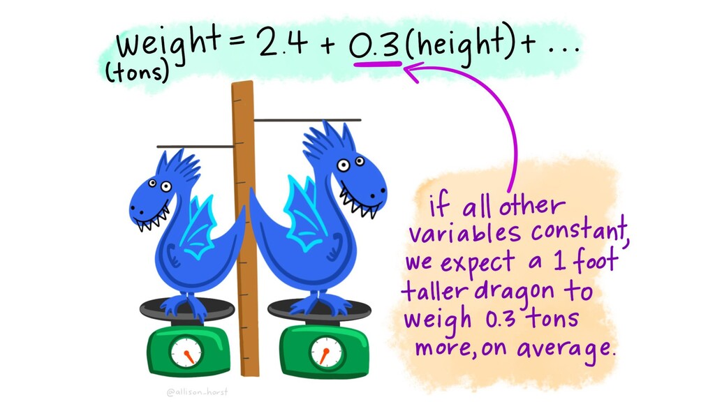
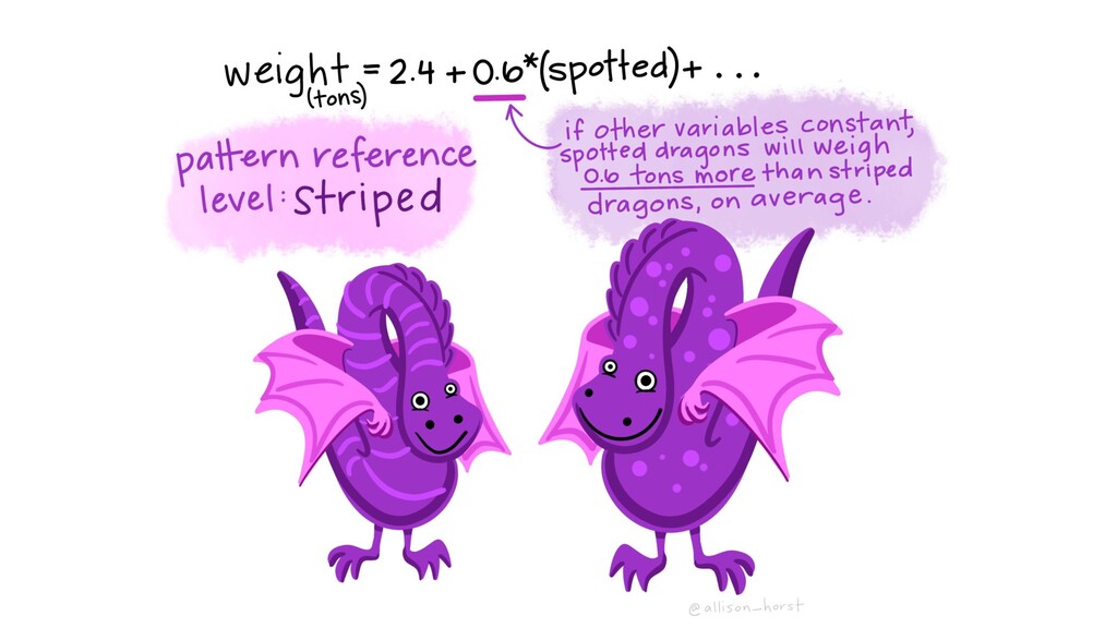
model” • Today’s Focus: Interpreting and specifying models. Not focusing on assessing fit whether the models are working. Y= βo + β1 X1 + β2 X2 … + error
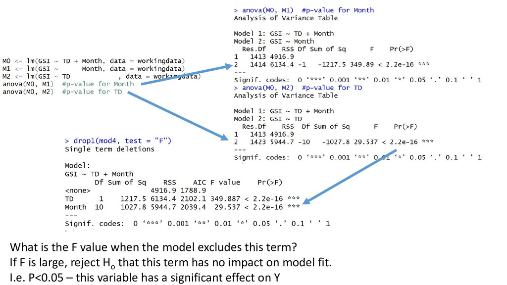
< 0.05. • If we repeated the study infinite times, we would erroneously reject Ho 5% of the time (i.e. we would conclude there IS an effect when one doesn’t exist, one time out of 20) • Every time you run a model you risk making this error • If you run multiple models, the risk of an error increases If both Site and TD matter, we should model them together. Why? Interpretability. Goal is not just to ask “is there an effect” – we want to measure magnitude of effect of each parameter. We want to see each variable’s contribution to changes in Y. Interaction. Covariates can impact Y on their own, or they can work in concert.
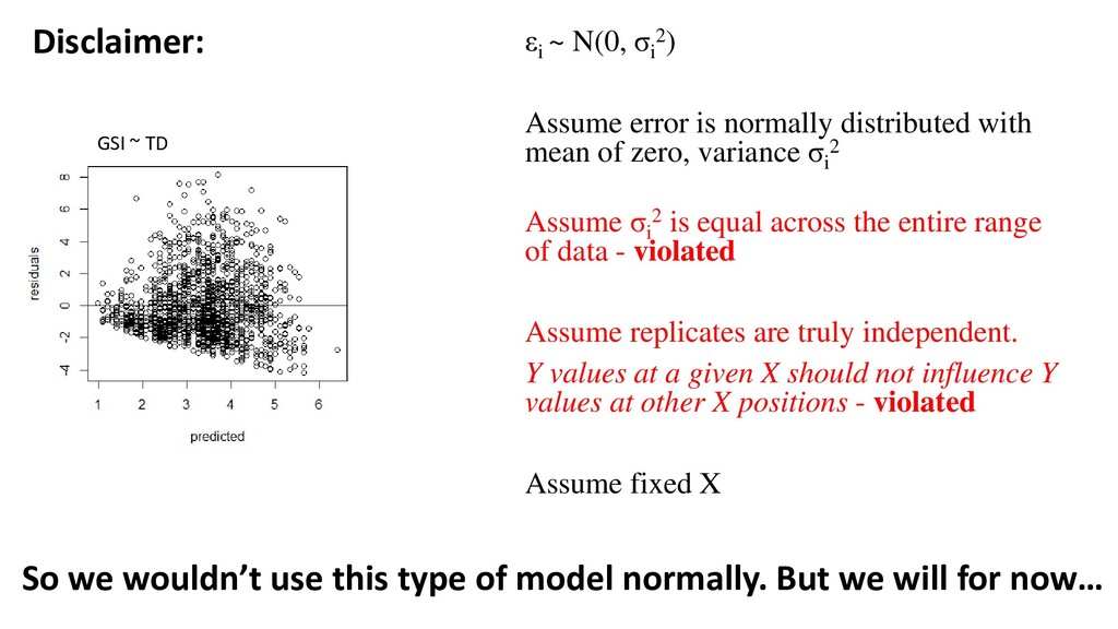
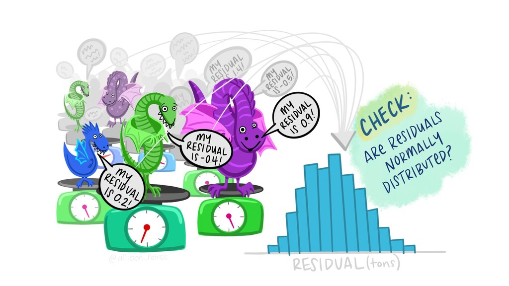
distributed with mean of zero, variance σi 2 Assume σi 2 is equal across the entire range of data - violated Assume replicates are truly independent. Y values at a given X should not influence Y values at other X positions - violated Assume fixed X GSI ~ TD So we wouldn’t use this type of model normally. But we will for now…
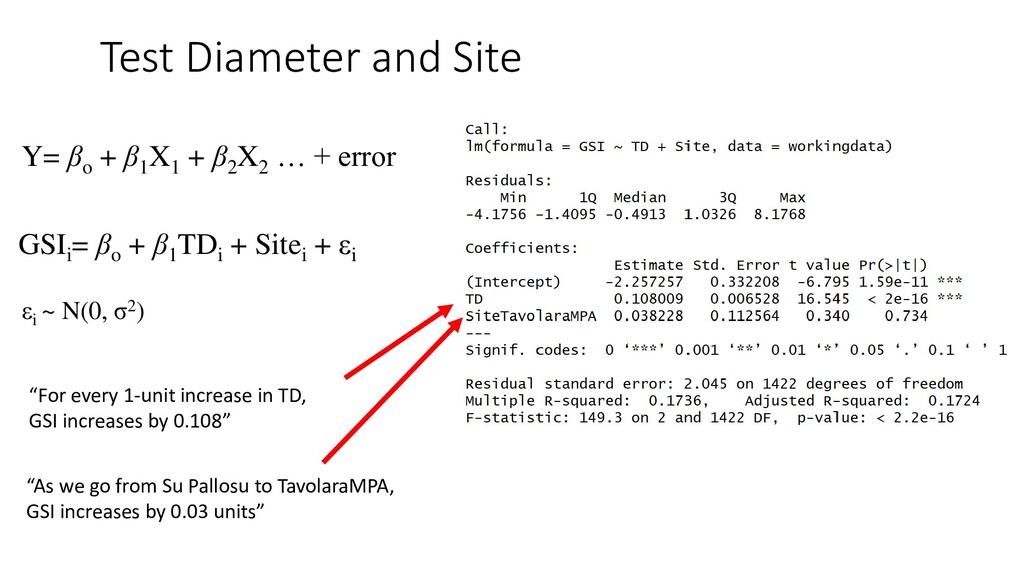
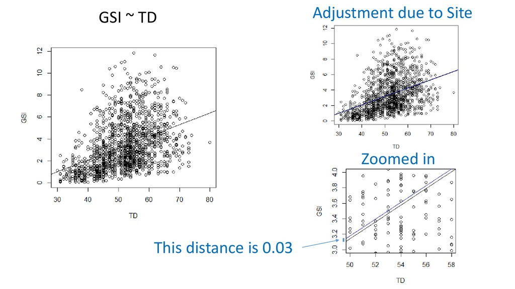
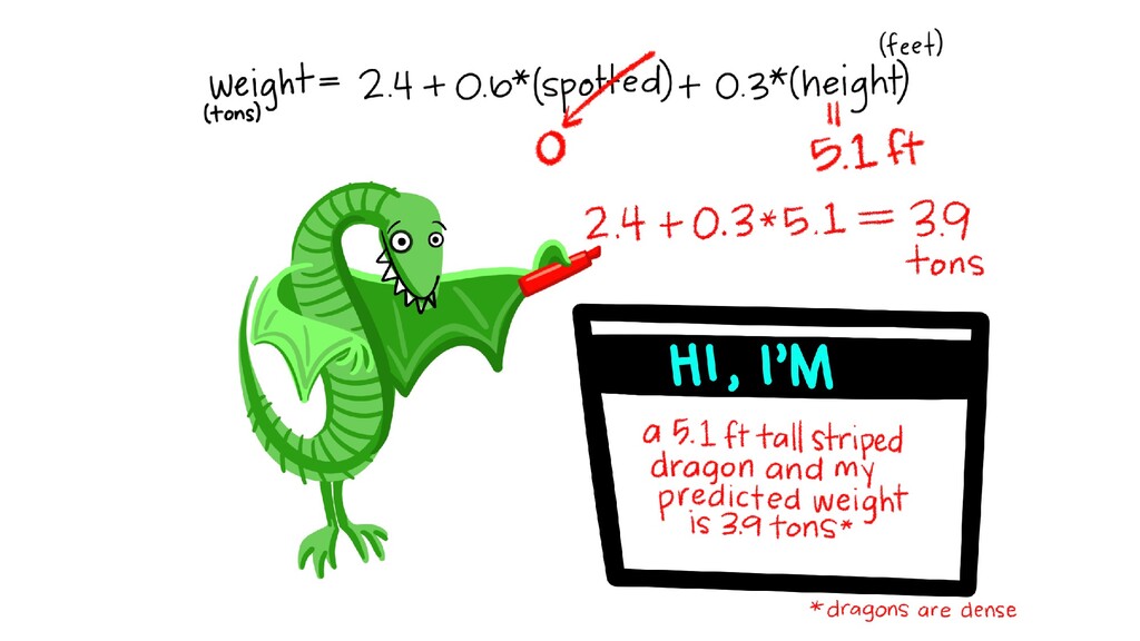
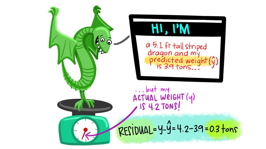
β2 X2 … + error GSIi = βo + β1 TDi + Sitei + εi εi ~ N(0, σ2) “For every 1-unit increase in TD, GSI increases by 0.108” “As we go from Su Pallosu to TavolaraMPA, GSI increases by 0.03 units”
GSIi = -2.26 + 0.108*TDi + 0 * SuPallosu + 0.0382 * TavolaraMPA + εi • When including a categorical covariate, by default, R makes all comparisons against the first alphabetical level in the factor • Here, “SuPallosu” comes before “TavolaraMPA” – so “SuPallosu” becomes default level • Implication: Control group should always be first level GSIi = β0 + β1 *TDi + 0 * SuPallosu + β2 * TavolaraMPA + εi
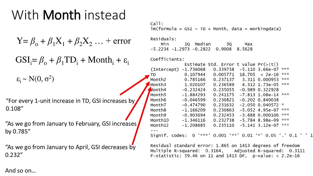
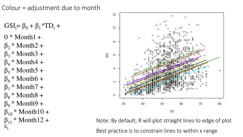
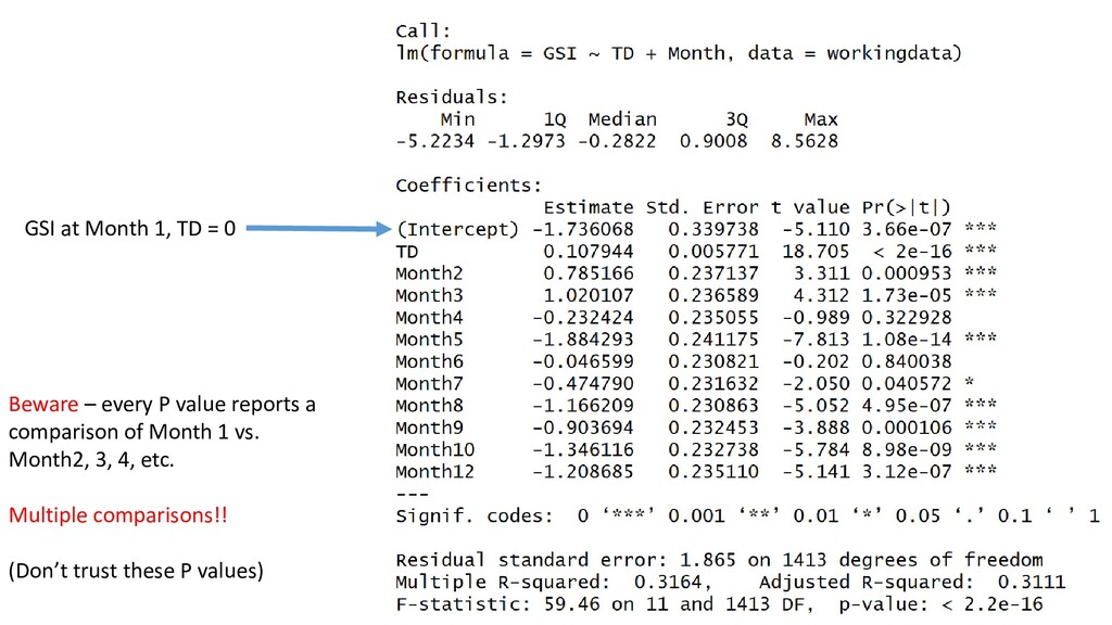
X2 … + error GSIi = βo + β1 TDi + Monthi + εi εi ~ N(0, σ2) “For every 1-unit increase in TD, GSI increases by 0.108” “As we go from January to February, GSI increases by 0.785” “As we go from January to April, GSI decreases by 0.232” And so on…
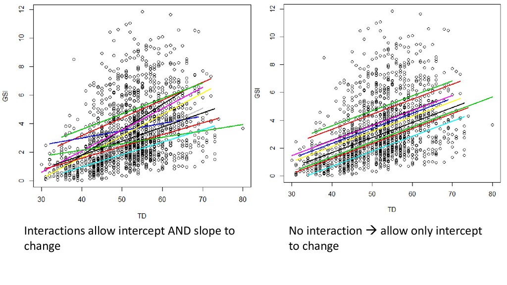
categorical variable bumps the line up and down • But what if we think the line is not only adjusted, but also has a different slope? • Consider Month * TD: GSIi = β0 + β1 TDi + Monthi + Month*TDi + εi
Month 1, every additional TD brings 0.179 units of increase in GSI As you go from Month 1 to Month 2, you see an increase of 3.54 in the intercept for GSI, when TD = 0 As you go from Month 1 to Month 2, subtract 0.054 from the base slope. In Month 2, for every additional unit of TD, you are getting 0.054 fewer units of increase in GSI 0.179 – 0.054 = 0.125 In Month 2, for every additional unit of TD, you get 0.125 units of GSI
Coefficients from summary() give you: • Intercept - Mean of the first level, all else being zero • Beta1 – difference between first level mean and second level • Beta2 – difference between first level mean and third level • Use drop1() or anova() to determine if the categorical covariate has an overall significant effect on Y • Both continuous and categorical covariates can be placed on X • Interactions allow slope to vary. No interaction = slope is constant across groups • Best to practice writing out all models that you run
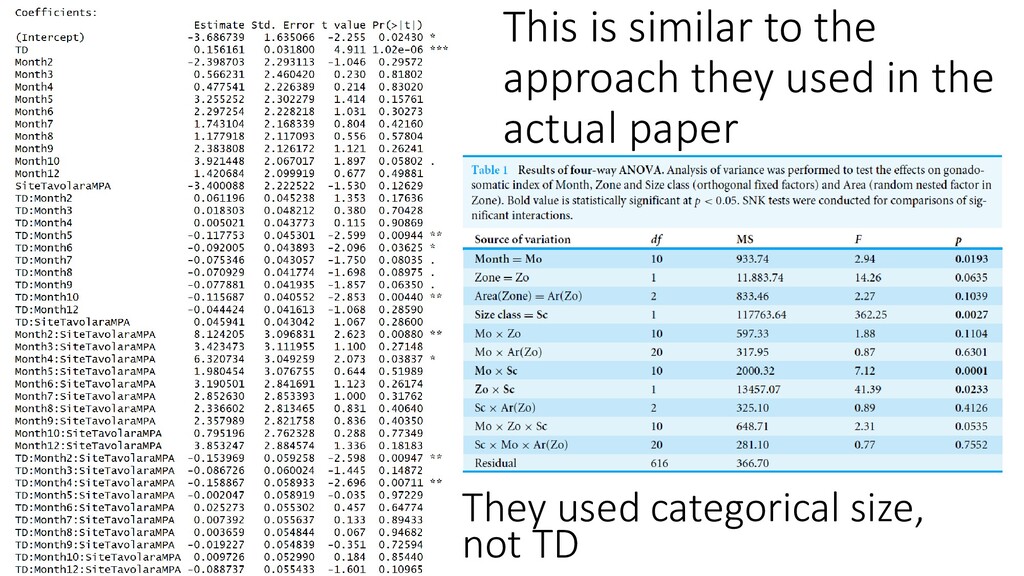
these P-values are assessing whether the significantly different levels of variance are explained by keeping the variable in the model. Low P-value = reject Ho that this variable has no effect on variance explained by model (They also used a random factor. We’ll talk about this later)
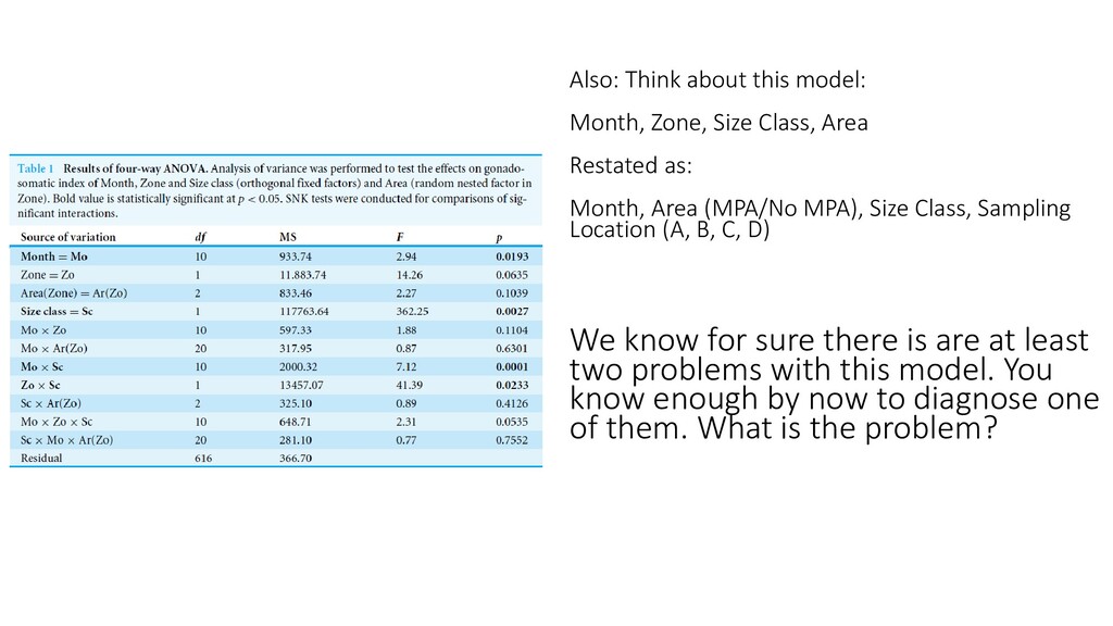
Restated as: Month, Area (MPA/No MPA), Size Class, Sampling Location (A, B, C, D) We know for sure there is are at least two problems with this model. You know enough by now to diagnose one of them. What is the problem?
in a model, with or without interactions • How to interpret betas – for both continuous and categorical covariates, as well as for interactions • Can build a model in R with one Y, and more than one covariate • Understand what Drop1 is doing Y= βo + β1 X1 + β2 X2 … + error εi ~ N(0, σ2)
Review and run 003_UrchinStats. This is code from TODAY’S lecture. • Note that we have not yet assessed whether any of these models are working (and we know that they probably aren’t). Next week. Tomorrow: • A big example, using a different study
) E(CatchRate) = μ ij Log(μ ij ) = GearType ij + Temperature ij + FleetDeployment i FleetDeployment i ~ N(0, σ2) Using lme4: m <- glmer(CatchRate ~ GearType + Temperature + (1 | FleetDeployment), family = poisson) FISH 6003 Part 2 FISH 6003: Statistics and Study Design for Fisheries Brett Favaro
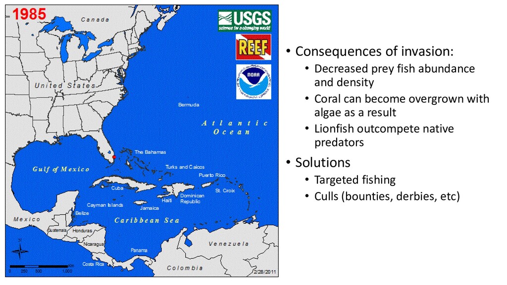
density • Coral can become overgrown with algae as a result • Lionfish outcompete native predators • Solutions • Targeted fishing • Culls (bounties, derbies, etc)
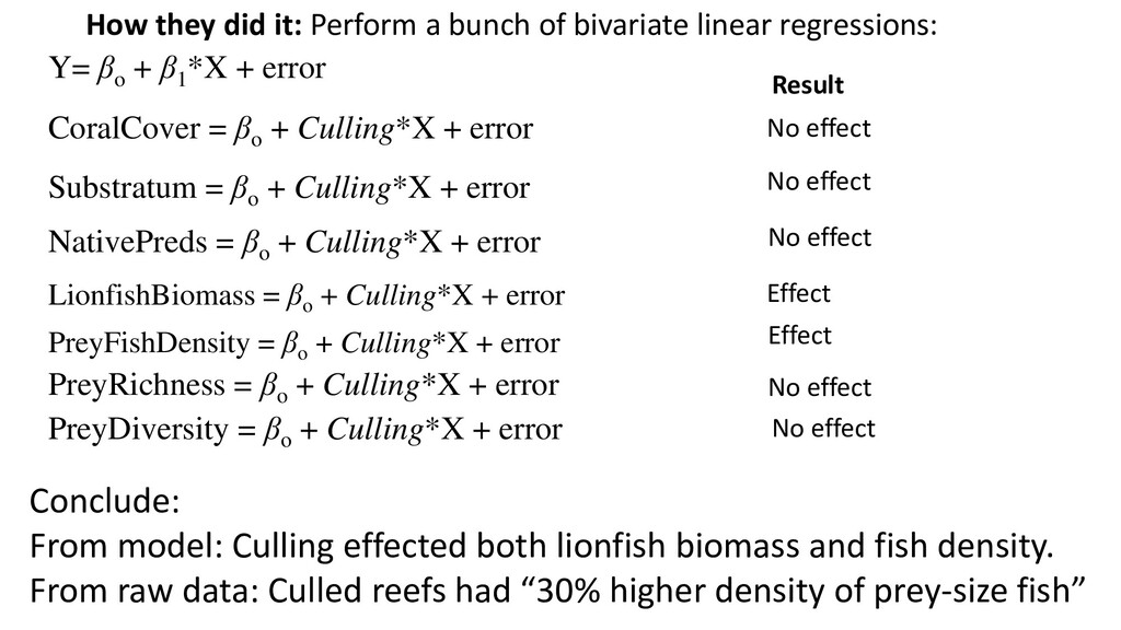
most pressing concerns in the context of coral reef conservation throughout the Caribbean. … In Roatan (Honduras) a local non-governmental organisation (i.e. Roatan Marine Park) trains residents and tourists in the use of spears to remove invasive lionfish. Here, we assess the effectiveness of local removal efforts in reducing lionfish populations. We ask whether reefs subject to relatively frequent removals support more diverse and abundant native fish assemblages compared to sites were no removals take place. Lionfish biomass, as well as density and diversity of native prey species were quantified on reefs subject to regular and no removal efforts. Reefs subject to regular lionfish removals (two to three removals month-1 ) with a mean catch per unit effort of 2.76 ± 1.72 lionfish fisher-1 h-1 had 95% lower lionfish biomass compared to nonremoval sites. Sites subject to lionfish removals supported 30% higher densities of native prey-sized fishes compared to sites subject to no removal efforts. We found no evidence that species richness and diversity of native fish communities differ between removal and non-removal sites. We conclude that opportunistic voluntary removals are an effective management intervention to reduce lionfish populations locally and might alleviate negative impacts of lionfish predation. We recommend that local management and the diving industry cooperate to cost-effectively extend the spatial scale at which removal regimes are currently sustained.
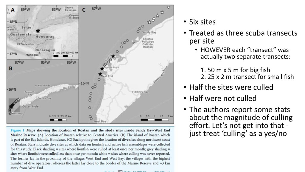
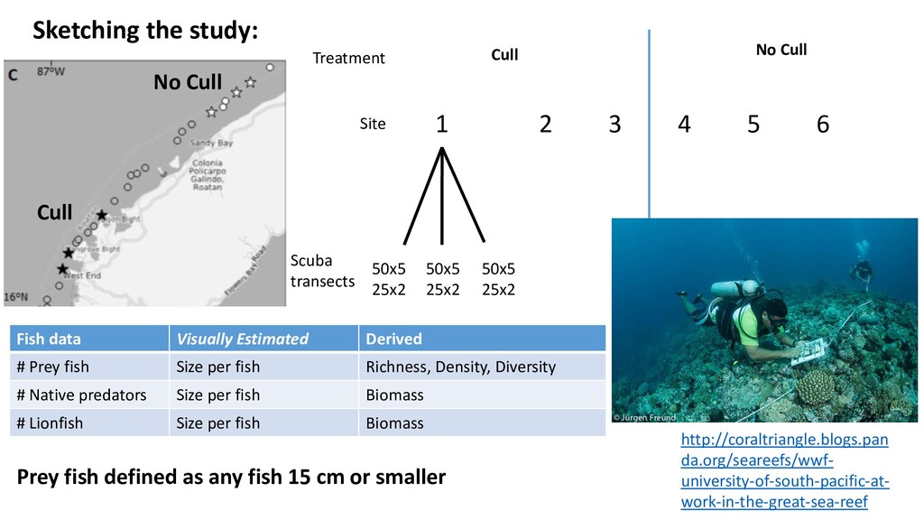
site • HOWEVER each “transect” was actually two separate transects: 1. 50 m x 5 m for big fish 2. 25 x 2 m transect for small fish • Half the sites were culled • Half were not culled • The authors report some stats about the magnitude of culling effort. Let’s not get into that - just treat ‘culling’ as a yes/no
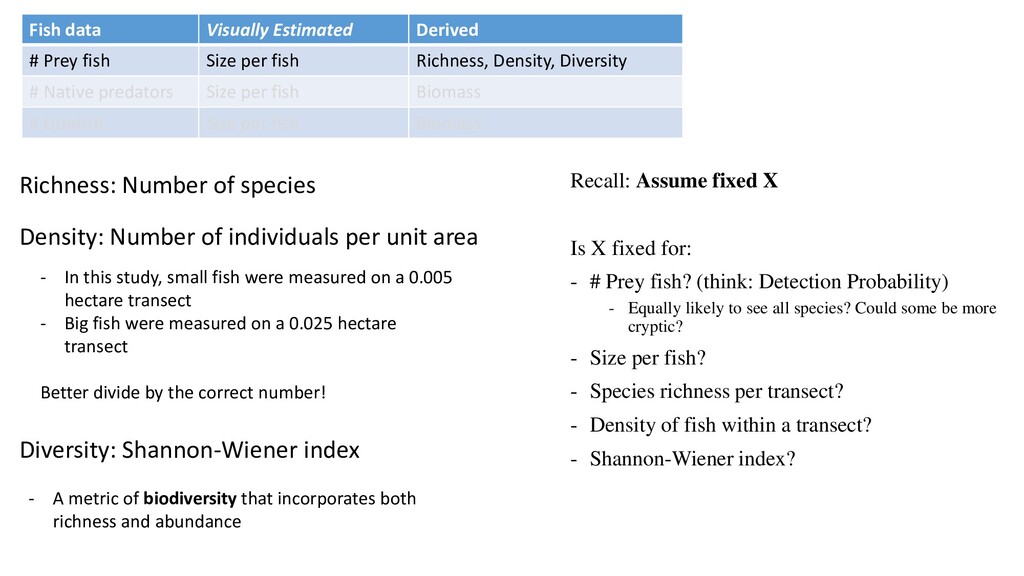
Treatment Cull No Cull Scuba transects 50x5 25x2 No Cull Cull 50x5 25x2 50x5 25x2 Fish data Visually Estimated Derived # Prey fish Size per fish Richness, Density, Diversity # Native predators Size per fish Biomass # Lionfish Size per fish Biomass http://coraltriangle.blogs.pan da.org/seareefs/wwf- university-of-south-pacific-at- work-in-the-great-sea-reef Prey fish defined as any fish 15 cm or smaller
fish Richness, Density, Diversity # Native predators Size per fish Biomass # Lionfish Size per fish Biomass Richness: Number of species Density: Number of individuals per unit area - In this study, small fish were measured on a 0.005 hectare transect - Big fish were measured on a 0.025 hectare transect Better divide by the correct number! Diversity: Shannon-Wiener index - A metric of biodiversity that incorporates both richness and abundance Recall: Assume fixed X Is X fixed for: - # Prey fish? (think: Detection Probability) - Equally likely to see all species? Could some be more cryptic? - Size per fish? - Species richness per transect? - Density of fish within a transect? - Shannon-Wiener index?
fish Richness, Density, Diversity # Native predators Size per fish Biomass # Lionfish Size per fish Biomass Biomass: Recall: Assume fixed X Is X fixed for: - # Native Predators? - Size per fish, for bigger fish? - Biomass? - Uncertainty around length-weight relationship? Is it consistent across body sizes? - Is uncertainty equivalent across species? Not given in the raw data, nor is it explained how they derived it for each fish Normally, you would use a published length-weight relationship: log(W) = log(a) + B*log(L) + error W is weight, L is length, and A and B are species-specific parameters Must disclose a and B! And beware; At extremes (especially low end) uncertainty increases with this translation
prey fish? • As defined by: • Species richness (# of species) • Shannon-Weiner index (calculated from # and abundance of species) • Abundance of prey fish? • Does culling lionfish decrease: • Density of lionfish? • But there are a lot of other variables • Site • Native predator density • Coral cover • Substratum complexity Q: What is truly driving the system?
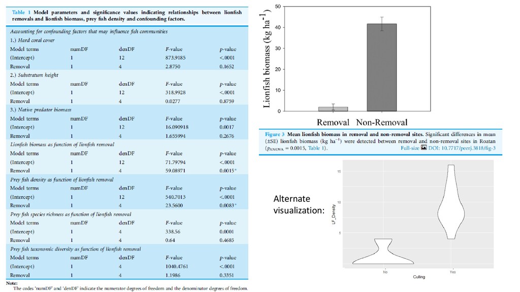
significant effect? Yes/no. P-value The raw data were used to answer: How much higher was reef density on these culled reefs? Danger: Multiple comparisons. Uncertainty on X due to derived values Missed opportunity: Use the MODEL to infer impact of culling on reef fish density – including 95% C.I. to tell us the magnitude of effect that was explainable by culling. If the model fits the data, this is powerful information!
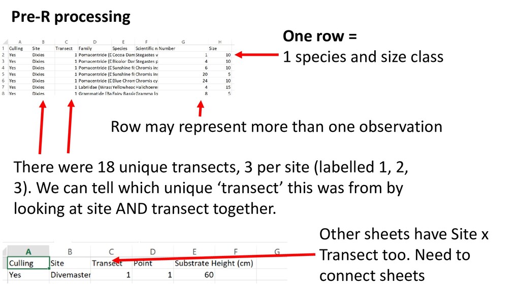
Row may represent more than one observation There were 18 unique transects, 3 per site (labelled 1, 2, 3). We can tell which unique ‘transect’ this was from by looking at site AND transect together. Other sheets have Site x Transect too. Need to connect sheets
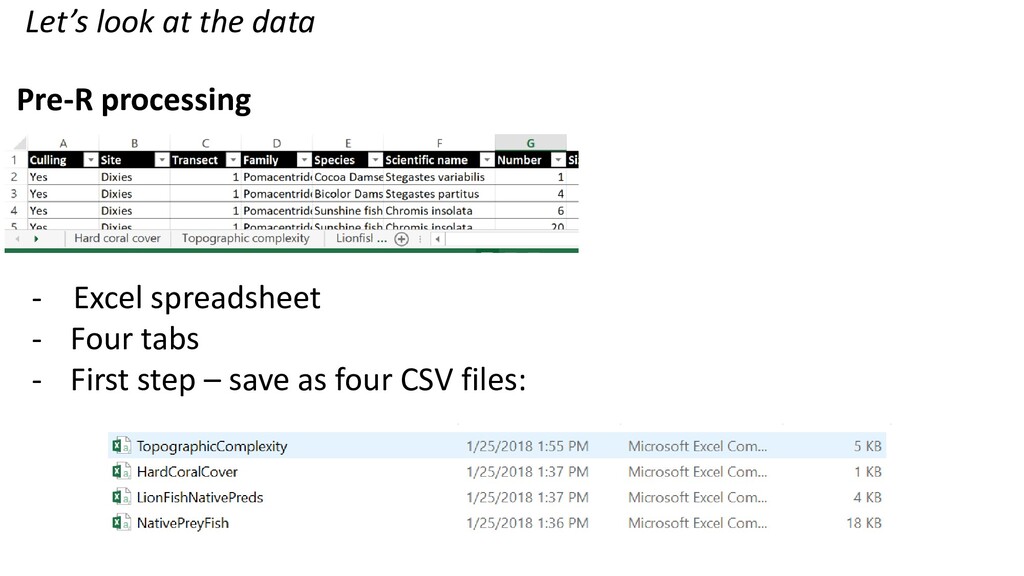
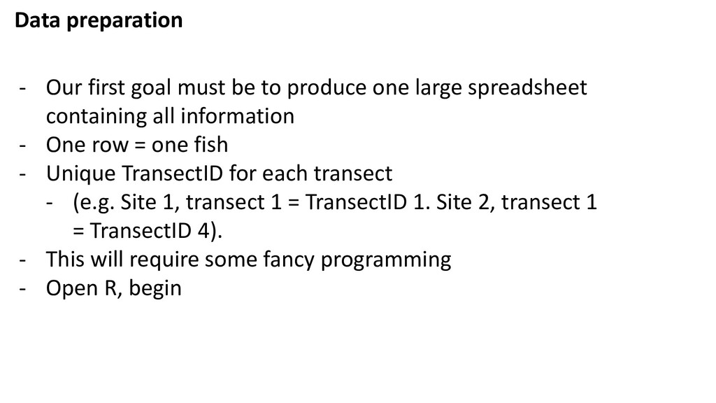
one large spreadsheet containing all information - One row = one fish - Unique TransectID for each transect - (e.g. Site 1, transect 1 = TransectID 1. Site 2, transect 1 = TransectID 4). - This will require some fancy programming - Open R, begin